Page 177 - Basic Structured Grid Generation

166 Basic Structured Grid Generation

and this is the Winslow model, eqns (5.1). Thus transformations satisfying the Winslow
model are extremals of the functional (6.41), which may be written, using (1.158),
(1.162), and (1.163), as
1 11 22
(g + g ) dx dy. (6.43)
2 R
Transforming the double integral to the computational domain gives
1 g 22 + g 11 √ 1 g 11 + g 22
( g dξ dη) = √ dξ dη. (6.44)
2 R g 2 R g
The Winslow transformation, mapping a square region to R, always gives an unfolded
grid, except for problems which can arise due to the nature of the discretization process
(i.e. truncation errors). In particular, this can happen when R is not convex.

6.4.2 The weighted L-functional

The concept of a weight function in one dimension can be generalized to higher
dimensions. Suppose that we wish the lengths of grid cells in the ξ and η directions
at a point corresponding to (ξ, η) in the computational plane to be proportional to the
positive weight functions ϕ(ξ, η), ψ(ξ, η), respectively. Then a functional analogous
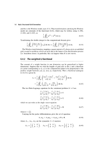
to (6.13) is given by

2
2
1 (x ξ ) + (y ξ ) 2 (x η ) + (y η ) 2
I L = + dξ dη
2 R ϕ(ξ, η) ψ(ξ, η)
1 g 11 g 22
= + dξ dη. (6.45)
2 R ϕ(ξ, η) ψ(ξ, η)
The two Euler-Lagrange equations for the variational problem δI = 0are
∂ 1 ∂x ∂ 1 ∂x
+ = 0
∂ξ ϕ ∂ξ ∂η ψ ∂η
∂ 1 ∂y ∂ 1 ∂y
+ = 0, (6.46)
∂ξ ϕ ∂ξ ∂η ψ ∂η
which we can write as the single vector equation

∂ 1 ∂r ∂ 1 ∂r
+ = 0, (6.47)
∂ξ ϕ ∂ξ ∂η ψ ∂η
x

where r = .
y
Carrying out the partial differentiations gives the set of equations
A 11 r ξξ + A 12 r ξη + A 22 r ηη + S = 0, (6.48)
where A 11 , A 12 , A 22 are the symmetric 2 × 2 matrices
1 10 00 1 10
A 11 = , A 12 = , A 22 = , (6.49)
ϕ 01 00 ψ 01