Page 172 - Basic Structured Grid Generation

Variational methods and adaptive grid generation 161

u

O
x x x x 3 x 4 x 5 x 6 x
0 1 2

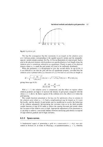
Fig. 6.2 Equidistant grid.

This has the consequence that the increments in arc-length on the solution curve
u(x) between points corresponding to the equally-spaced ξ points and the unequally-
spaced x points remain constant. See Fig. 6.2 for an illustration of a typical grid. Such a
grid in the physical domain which produces an equidistribution of arc-length along the
solution curve is sometimes referred to as equidistant. Clearly in parts of the physical
domain where u x is small the grid points will tend to be uniformly distributed.
When the parameter α is incorporated to give the second choice in eqn (6.24), it
is not difficult to see that the grid still has an equidistant property, provided that the
solution curve is plotted with u as a function of x/α. For then we can write arc-length as

du
2
2
2
s
d˜ = 1 + d(x/α) = 1 + α (u x ) d(x/α) = W(x) d(x/α),
d(x/α)
giving from eqn (6.21)
s
d˜ dx d˜ s
= α = K.
d(x/α) dξ dξ
With α> 1, the solution curve is compressed, and the effect on regions where
solution gradients are high is to increase the density of grid-points compared with the
choice α = 1 above. In flatter regions of the solution curve the effect is to widen the
grid-spacing.
The weight functions presented so far may not be satisfactory close to extrema in
the solution curve where u x = 0. Such a neighbourhood may be treated as if it were
flat locally, and the density of grid points may be insufficient to resolve the behaviour
of the solution adequately. Incorporating the curvature term as in the third possible
weight function of eqn (6.24) tends to reduce the spacing between grid points where
the curvature of the solution curve is high. Appropriate adjustment of the parameters α,
β can help to achieve a successful balance between increasing grid-density in regions
of high solution gradient and of high curvature.

6.3.3 Space-curves

A fundamental aspect of generating a grid on a space-curve r = r(χ) was pre-
sented in Section 2.4. in terms of obtaining a re-parameterization χ → ξ, whereby