
Page 171 - Basic Structured Grid Generation
P. 171
160 Basic Structured Grid Generation
particular where the first derivative u x (= du/dx) has a high value so that grid-points
locally are close together. The most commonly used weight functions are
u x (x)
2
W (x) = 1 + α (u x ) 2 (6.24)
(1 + βκ) 1 + α (u x ) ,
2 2
similar to the expressions given in eqns (2.58), (2.59), and (2.60), where here κ is the
curvature of the solution, given by
|u xx |
κ = (6.25)
2 3/2
[1 + (u x ) ]
as in eqn (2.17), and α, β are parameters to be chosen by the user.
Note that with W(x) = u x , eqn (6.21) becomes
du dx du
= = K, (6.26)
dx dξ dξ
which has the consequence that the increments in the values of u between the equally-
spaced points on the ξ interval and between the corresponding unequally-spaced grid
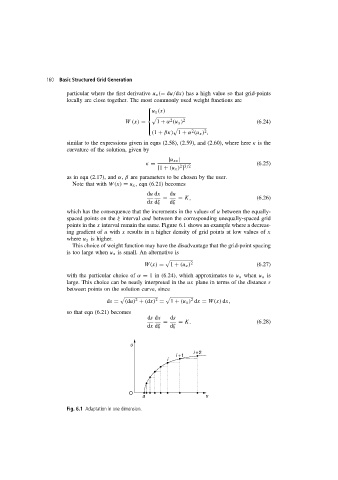
points in the x interval remain the same. Figure 6.1 shows an example where a decreas-
ing gradient of u with x results in a higher density of grid points at low values of x
where u x is higher.
This choice of weight function may have the disadvantage that the grid-point spacing
is too large when u x is small. An alternative is
W(x) = 1 + (u x ) 2 (6.27)
with the particular choice of α = 1 in (6.24), which approximates to u x when u x is
large. This choice can be neatly interpreted in the ux plane in terms of the distance s
between points on the solution curve, since
2 2 2
ds = (du) + (dx) = 1 + (u x ) dx = W(x) dx,
so that eqn (6.21) becomes
ds dx ds
= = K. (6.28)
dx dξ dξ
u
i +2
i +1
i
O
a x
Fig. 6.1 Adaptation in one dimension.