Page 176 - Basic Structured Grid Generation

Variational methods and adaptive grid generation 165

will help readers to write their own programs to generate grids for different geometries
to match particular requirements.)

6.4.1 The L-functional and the Winslow model

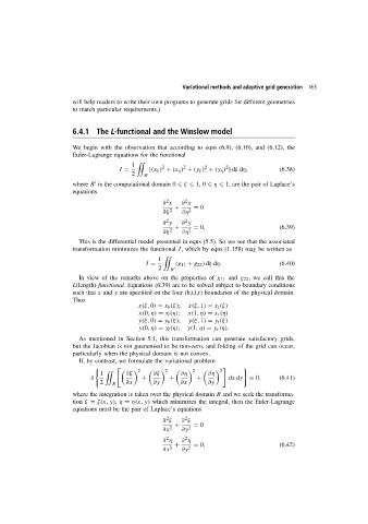
We begin with the observation that according to eqns (6.9), (6.10), and (6.12), the
Euler-Lagrange equations for the functional
1 2 2 2 2
I = {(x ξ ) + (x η ) + (y ξ ) + (y η ) } dξ dη, (6.38)
2 R

where R is the computational domain 0 ξ 1, 0 η 1, are the pair of Laplace’s
equations
2
2
∂ x ∂ x
+ = 0
∂ξ 2 ∂η 2
2
2
∂ y ∂ y
+ = 0. (6.39)
∂ξ 2 ∂η 2
This is the differential model presented in eqns (5.5). So we see that the associated
transformation minimizes the functional I, which by eqns (1.158) may be written as
1
I = (g 11 + g 22 ) dξ dη. (6.40)
2 R
In view of the remarks above on the properties of g 11 and g 22 , we call this the
L(length)-functional. Equations (6.39) are to be solved subject to boundary conditions
such that x and y are specified on the four (b,t,l,r) boundaries of the physical domain.
Thus
x(ξ, 0) = x b (ξ); x(ξ, 1) = x t (ξ)
x(0,η) = x l (η); x(1,η) = x r (η)
y(ξ, 0) = y b (ξ); y(ξ, 1) = y t (ξ)
y(0,η) = y l (η); y(1,η) = y r (η).
As mentioned in Section 5.1, this transformation can generate satisfactory grids,
but the Jacobian is not guaranteed to be non-zero, and folding of the grid can occur,
particularly when the physical domain is not convex.
If, by contrast, we formulate the variational problem
2 2 2 2
1 ∂ξ ∂ξ ∂η ∂η
δ + + + dx dy = 0, (6.41)
2 R ∂x ∂y ∂x ∂y
where the integration is taken over the physical domain R andweseekthe transforma-
tion ξ = ξ(x, y), η = η(x, y) which minimizes the integral, then the Euler-Lagrange
equations must be the pair of Laplace’s equations
2
2
∂ ξ ∂ ξ
+ = 0
∂x 2 ∂y 2
2
2
∂ η ∂ η
+ = 0, (6.42)
∂x 2 ∂y 2