Page 174 - Basic Structured Grid Generation

Variational methods and adaptive grid generation 163

Here we have
2
2
˜ g 11 = 1 + (1 − 2χ) = 2 − 4χ + 4χ . (6.35)
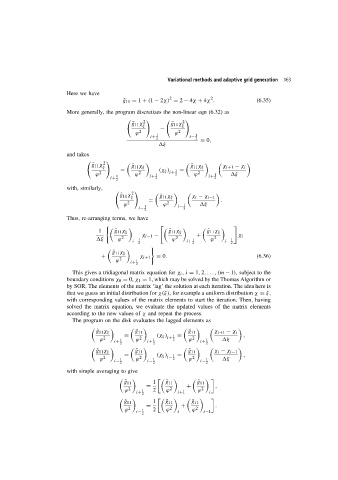
More generally, the program discretizes the non-linear eqn (6.32) as
2
2
˜ g 11 χ ˜ g 11 χ
ξ ξ
−
ϕ 2 1 ϕ 2 1
i+ i−
2 2 = 0,
ξ
and takes
2
˜ g 11 χ
ξ ˜ g 11 χ ξ ˜ g 11 χ ξ χ i+1 − χ i
= (χ ξ ) 1 =
ϕ 2 ϕ 2 1 i+ 2 ϕ 2 1 ξ
i+ 1 i+ 2 i+ 2
2
with, similarly,
2
˜ g 11 χ
ξ ˜ g 11 χ ξ χ i − χ i−1
= .
ϕ 2 ϕ 2 1 ξ
i− 1 i− 2
2
Thus, re-arranging terms, we have

1 ˜ g 11 χ ξ ˜ g 11 χ ξ ˜ g 11 χ ξ
χ i−1 − + χ i
ξ ϕ 2 1 ϕ 2 1 ϕ 2 1
i− i+ i−
2 2 2

˜ g 11 χ ξ
+ χ i+1 = 0. (6.36)
ϕ 2 1
i+
2
This gives a tridiagonal matrix equation for χ i , i = 1, 2,...,(m − 1), subject to the
boundary conditions χ 0 = 0, χ 1 = 1, which may be solved by the Thomas Algorithm or
by SOR. The elements of the matrix ‘lag’ the solution at each iteration. The idea here is
that we guess an initial distribution for χ(ξ), for example a uniform distribution χ = ξ,
with corresponding values of the matrix elements to start the iteration. Then, having
solved the matrix equation, we evaluate the updated values of the matrix elements
according to the new values of χ and repeat the process.
The program on the disk evaluates the lagged elements as

˜ g 11 χ ξ ˜ g 11 ˜ g 11 χ i+1 − χ i
= (χ ξ ) 1 = ,
ϕ 2 1 ϕ 2 1 i+ 2 ϕ 2 1 ξ
i+ i+ i+
2 2 2

˜ g 11 χ ξ ˜ g 11 ˜ g 11 χ i − χ i−1
= (χ ξ ) 1 = ,
ϕ 2 1 ϕ 2 1 i− 2 ϕ 2 1 ξ
i− i− i−
2 2 2
with simple averaging to give

˜ g 11 1 ˜ g 11 ˜ g 11
= + ,
ϕ 2 1 2 ϕ 2 ϕ 2
i+ i+1 i
2

˜ g 11 1 ˜ g 11 ˜ g 11
= + .
ϕ 2 1 2 ϕ 2 ϕ 2
i− i i−1
2