Page 28 - Basic Structured Grid Generation

Mathematical preliminaries – vector and tensor analysis 17

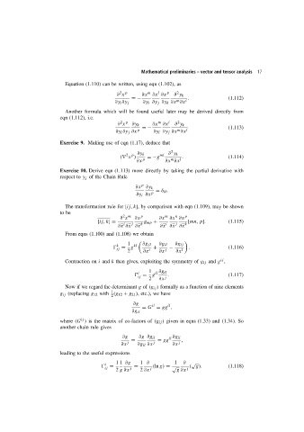
Equation (1.110) can be written, using eqn (1.102), as
l
m
2
2 p
∂ x ∂x ∂x ∂x p ∂ y k
=− m l . (1.112)
∂y i ∂y j ∂y i ∂y j ∂y k ∂x ∂x
Another formula which will be found useful later may be derived directly from
eqn (1.112), i.e.
m
2 p
2
∂ x ∂y k ∂x ∂x l ∂ y k
=− (1.113)
m
∂y i ∂y j ∂x p ∂y i ∂y j ∂x ∂x l
Exercise 9. Making use of eqn (1.17), deduce that
2
2 p ∂y k ml ∂ y k
(∇ x ) =−g . (1.114)
m
∂x p ∂x ∂x l
Exercise 10. Derive eqn (1.113) more directly by taking the partial derivative with
respect to y j of the Chain Rule
p
∂x ∂y k
= δ ik .
∂y i ∂x p
The transformation rule for [ij, k], by comparison with eqn (1.109), may be shown
to be
m
2 m
n
∂ x ∂x p ∂x ∂x ∂x p
[ij, k]= i j k g mp + i j k [mn, p]. (1.115)
∂x ∂x ∂x ∂x ∂x ∂x
From eqns (1.100) and (1.108) we obtain
1
k kl ∂g jl ∂g il ∂g ij
= g + − . (1.116)
ij
2 ∂x i ∂x j ∂x l
ij
Contraction on i and k then gives, exploiting the symmetry of g ij and g ,
1
i il ∂g il
= g . (1.117)
ij j
2 ∂x
Now if we regard the determinant g of (g ij ) formally as a function of nine elements
1
g ij (replacing g 12 with (g 12 + g 21 ),etc.), we have
2
∂g il il
= G = gg ,
∂g il
ij
where (G ) is the matrix of co-factors of (g ij ) given in eqns (1.33) and (1.34). So
another chain rule gives
∂g ∂g ∂g il il ∂g il
= = gg ,
∂x j ∂g il ∂x j ∂x j
leading to the useful expressions
1 1 ∂g 1 ∂ 1 ∂ √
i
= = (ln g) = √ ( g). (1.118)
ij j j j
2 g ∂x 2 ∂x g ∂x