Page 134 - Basic Well Log Analysis for Geologist

LITHOLOGY LOGGING AND MAPPING TECHNIQUES

en a

(sucrosic and intergranular). A crossplot of these two MID* Lithology Plot
variables makes lithology more apparent. M* and N* values ,
The MID* (Matrix Identification) plot, like the M-N* isa
are calculated by the following equations (Schlumberger,
crossplot technique which helps identify lithology and
1972):
secondary porosity. Also, like the M-N* plot, the MID*
Mt = Ate — At x 0.01 plot requires data from neutron, density, and sonic logs.
Po — Pr
The first step in constructing a MID* plot is to determine
values for the apparent matrix parameters (Pia), and
—
N*¥ = Ont > On,
(Atwa)a- These values are determined from neutron (by).
Po ~ Pt
density (p,), and sonic (At) data obtained from the log.
Next, these values (i.e. fy, pp. and At) are crossplotted on
At; = interval transit time of fluid (189 for fresh mud
appropriate neutron-density and sonic-density charts to
und 185 for salt mud)
obtam (Pm) and (Aty,y)a Values. Crossplot charts, along
At = interval transit time from the log
with instructions on how to use them, can be obtained from
pr = density of fluid (1.0 for fresh mud and 1.1 for salt
Schlumberger’s Log Interpretation Mauual/Applications.,
inud)
Volume II (1974). The method for obtaining apparent
Py» = bulk density of formation
matrix parameters (Py), and (At), is also
(x = neutron porosity of the formation from
illustrated in the case studies discussed in Chapter VIL.
Conipensated Neutron or Sidewall Neutron
Once obtained, apparent matrix parameters
Porosity Log
(Pma)a and (At,,,), are plotted on the MID* plot (Fig. 47).
dye = neutron porosity of fluid (use 1.0)
Data plotted in Figure 47 arerom the Alpar Resources
When the matrix parameters (Atma, Pma: PNma; Table [0) Federal 1-10 well, Richland County, Montana (Fig. 45),
are used in the M* and N* equations instead of formation and include the same Red River C-zone interval (11.870 to
parameters, M* and N* values can be obtained for the 11.900 ft) iNustrated in the M-N* plot (Fig. 46). The data
various minerals (Table 11). points form a cluster (Fig. 47) defined by the end-members:
Figure 46 is a M-N* plot of data from the Ordovician Red anhydrite, dolomite, and limestone. The lithology is an
vugs and/or fractures. Alpha Mapping from SP Log
River C-zone in the Alpar Resources Federal |-10,
anhydritic limey dolomite. The three points that plot above
the dolomite-limestone line indicate secondary porosity.
Richland County, Montana at a depth of 11,870 to 11,900 ft
(Fig. 45). Data from this interval, cluster together in the
M-N* lithology triangle. Lithology is defined by the
end-members: anhydrite, dolomite, and limestone. In this
case. lithology is an anhydritic limey dolomite (Fig. 46).
The spontaneous potential (SP) log (Chapter I) cun be
used to map clean sands (shale-free) versus shaly sands.
Notice that two of the data points are above the
The technique is called Alpha mapping (qa; Dresser Atlas,
dolomite-limestone line, indicating secondary porosity from
1974), and is based on the observation that the presence of
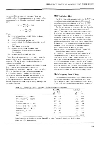
Table 11. Values of M* and N* constants, calculated for Common Minerals.

Fresh Mud Salt Mud
(p = 1.0) (p= 1.1)
Me N*M ONE

Sandstone (1) Vijg = 18,000 810.628 835.669
Sandstone (2) Ving = 19.500 .835 628 862.669
Limestone 827.585 854.621
Dolomite (1) @ = 3.5 — 30% 778 516 800 544
Dolomite (2) @ = 1.5 — 5.5% 778.524 O00 554
Dolomite (3) @ = 0 — 1.5% 778 532 800.561
Anhydrite p,,, = 2.98 702.505 718.532
Gypsum 1.015 .378 1.064.408
Salt 1.269 1.032

From Schlumberger Log Interpretation Manual/Principles. Courtesy Schlumberger Well Services;
Copyright 1972, Schlumberger.

119