Page 130 - Basic Well Log Analysis for Geologist

LOG INTERPRETATION

verre

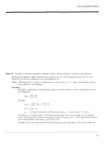
Figure 43. Example of a resistivity versus porosity (Hingle) crossplot. Morrow sandstone, Cimarron County, Oklahoma.
Before using the Hingle crossplot to determine water saturation (S,,) for a well-completion decision (see text, steps |
through 8), you must first calibrate the x-axis scale for porosity (#).
Given: Fluid density (p,) = 1.0 gm/cc for freshwater mud; matrix density (pma) = 2.7 gm/ce (from Hingle crossplot);
derived porosity is 10% (arbitrary).

Procedure:
Remember that the density of derived porosity (dpe,) is calculated as follows (see text, under heading: Density
Log; Chapter IV):
pen — Pma~ Po
Pma — Pf
Therefore:
2.70 — py 2.70
py
—
0.10 = > =
10 2.70 — 1.0 1.7
0.17 = 2.70 — p,
Py = 2.53 gm/cc bulk density at 10% porosity when py, = 2.7 gm/ce and pr = 1.0 gm/cc
The values py, = 2.53 gm/cc and @ = 10% should coincide on the x-axis. In step 2 of the text, you scaled the
x-axis. This exercise (Fig. 43) gives you one point on your x-axis (p, at 2.53; b = 10%): steps 4 and 5 in the text
give you the end-point of your scale (p,,, at 2.70: @ = 0%).
Scale the x-axis to cover values between 0% and 10% porosity, and continue above 10% to the end of the chart.

115