Page 84 - Basics of Fluid Mechanics and Introduction to Computational Fluid Dynamics

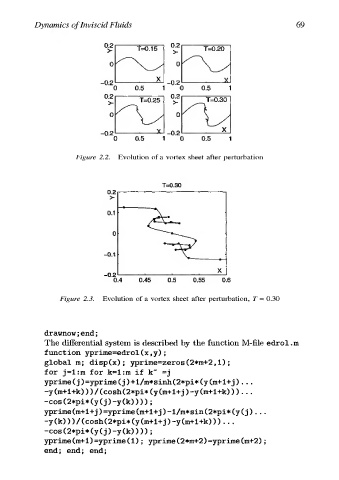
Dynamics of Inviscid Fluids 69

T=0.15 | %?
Oe
T=0.20
aN K \

x
-0.2
XI _g2
o of 1 0 oO8 1
02 0.2
> T=0.25 | > T=0.30
;
O hom» Sw
-0.2 x

1
0.5 x! _o2 1
0
0.5
Figure 2.2. Evolution of a vortex sheet after perturbation

T=0.30

x

0.4 0.45 0.5 0.55 0.6

Figure 2.3. Evolution of a vortex sheet after perturbation, 7 = 0.30

drawnow;end;
The differential system is described by the function M-file edrol .m
function yprime=edrol (x,y);
global m; disp(x); yprime=zeros(2*m+2,1);

for j=i:m for k=1:m if k” =j
yprime (j)=yprime (j)+1/m*sinh(2*pix(y (m+i+j)...
~y (mt+it+k) ))/(cosh(2*pi*
(Cy Gnt+i+j)-y (mtitk)))...
-cos(2*pi*(y(j)-y(k))));
yprime(m+1+j)=yprime (m+1+j)—-1/m*sin(2*pi*(y(j)...
-y (k)))/(cosh(2*pix (Cy (m+1+j)-y(mtitk)))...
-—cos(2*pi*(y(j)-y(k))));
yprime (m+1)=yprime(1); yprime(2*m+2)=yprime (mt2) ;

end; end; end;