Page 83 - Basics of Fluid Mechanics and Introduction to Computational Fluid Dynamics

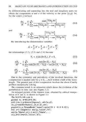
68 BASICS OF FLUID MECHANICS AND INTRODUCTION TO CFD

by differentiating and separating into the real and imaginary parts we

obtain the components u and v of the velocity at the point (z,y). So,
for the vortex 7 we have

dey usin 27 (Yj —Yx) oo
m

dt m kz) cosh [ee] ~ cos [aye]

and on
(Lj —Lp
dys UE y . (2.4)
a
dt ™m ray cosh jawed ~ COB [eee

By introducing the dimensionless variables

L y a tu

’ r’ ’ mA

the relationships (2.2), (2.3) and (2.4) become

Y; = Asin (27X,;),T =0, (2.5)

aX; 1 s sinh [2m (Yj — Yx)] (2.6)

dT mm wy cosh [27 (Y; — Yx)] — cos [2a (Xj — Xx)]’

dT ™m™ i cosh [2m (Y; — Y;)] — cos [2a (Xj; — Xx)]

Due to the symmetry and periodicity of the involved functions, the

computation is needed only for 7 = 2,...,m/2 within a half of the wave-
length. The greatest part of this computation involves the above Cauchy
problem numerically solving.
The computer result is an animation which shows the evolution of the
perturbation in time (see also Figure 2.2).
An enlarged picture of the interest zone, obtained by cubical interpo-

lation of X and Y, is shown in Figure 2.3.
The MATLAB code is
global m; m=40;A=0.05;
x=0:1/m:1;y=A*sin(2*pi*x); u0=[x;y];
[t ,u] =ode45(@edrol, [0,0.3] ,u0);
p=plot (x,y,’/EraseMode’,’none’) ;axis([0 1 -0.3 0.3]);
;
for j=1:length(t) set(p,’color’,'w’)
set (p,/Xdata’,u(j,i:mti) ,’Ydata’,...
u(j ,m+2:2*m+2) ,'’color’ ,’k’) ;