Page 181 - Biomimetics : Biologically Inspired Technologies

Bar-Cohen : Biomimetics: Biologically Inspired Technologies DK3163_c005 Final Proof page 167 6.9.2005 12:11pm

Genetic Algorithms in Optimization Models 167

5.4.1 The Genetic Algorithm Process

For the illustrative genetic algorithm problem (post office branches), we selected the following
parameters. We maintain a population of five members. The parents are randomly selected to
produce an offspring. An offspring replaces the worst population member if (a) it is better than the
worst population member and (b) it is not identical to an existing population member. The merging
rule is as follows: the two parents are compared and all variables (genes) common to both retain this
common value. For the variables with different values (one parent has a ‘‘0’’ and the other has a
‘‘1’’), we randomly select the necessary number of ‘‘1’’s to bring the total number of ‘‘1’’s to 3.
Thus, the offspring satisfies Equations (5.2) and (5.3). For example, the two parents are 1001001
and 0111000. We first determine the common genes creating 0111001 )***100*, where an asterisk
1001000
denotes an undetermined value which may be either ‘‘0’’ or ‘‘1.’’ Two ‘‘1’’s out of the four ‘‘*’’s are
randomly selected, while the rest get a ‘‘0.’’ The first two stars were randomly selected as ‘‘1’’s, and
the offspring is therefore 1101000. Its value of the fit function is calculated by Equation (5.1). This
process closely simulates nature with one exception. In the algorithm, if both parents have the same
trait for a specific gene, it is passed on to the offspring. If they have different traits, one of them
is randomly selected for the offspring. In nature, half of each chromosome is passed on to the
offspring. Also, there are dominant and recessive genes that determine the trait of the offspring.
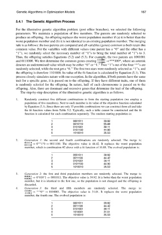
The step-by-step description of the illustrative genetic algorithm is as follows.

1. Randomly construct five different combinations to form the starting population (we employ a
population of five members). Next to each member is its value of the objective function calculated
by Equation (5.1). Since there are only 35 possible combinations we can construct them all and take
the fit function values from Table 5.2. Typically, such a table cannot be constructed and the fit
function is calculated for each combination separately. The random starting population is:

1 0001011 39.92
2 0010110 55.88
3 0101001 39.11
4 0101100 44.90
5 1010010 35.53
2. Generation 1: the second and fourth combinations are randomly selected. The merge is:
0010110 ) 0
1 0 ) 0011100. The objective value is 44.42. It replaces the worst population
0101100
member, which is combination #2 above with a fit function of 55.88. The evolved population is:
1 0001011 39.92
2 0011100 44.42
3 0101001 39.11
4 0101100 44.90
5 1010010 35.53
3. Generation 2: the first and third population members are randomly selected. The merge is:
0001011 ) 0 010 1 ) 0001011. The objective value is 39.92. It is better than the worst population

0101001
member, but it is identical to the first one, so the population is not changed and the offspring is
discarded.
4. Generation 3: the third and fifth members are randomly selected. The merge is:
0101001 ) ) 1010001. The objective value is 31.01. It replaces the worst population
0
1010010
member, the fourth one. The evolved population is:
1 0001011 39.92
2 0011100 44.42
3 0101001 39.11
4 1010001 31.01
5 1010010 35.53