Page 96 - Biomimetics : Biologically Inspired Technologies

Bar-Cohen : Biomimetics: Biologically Inspired Technologies DK3163_c003 Final Proof page 82 21.9.2005 11:40pm

82 Biomimetics: Biologically Inspired Technologies

3.4.2 Segmenting the Attended Speaker and Recognizing Words

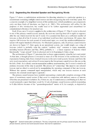
Figure 3.7 shows a confabulation architecture for directing attention to a particular speaker in a
soundstream containing multiple sound sources and also recognizing the next word they speak. For
a concrete example of a simplified version of this architecture (which nonetheless can competently
carry out these kinds of functions; see Sagi et al., 2001). This architecture will suffice for the
purposes of this introduction; but would need to be further augmented (and streamlined for
computational efficiency) for practical use.
Each 10 ms a new S vector is supplied to the architecture of Figure 3.7. This S vector is directed
to one of the primary sound lexicons; namely, the next one (moving from left to right) in sequence
after the one which received the last S vector. It is assumed that there are a sufficient number of
lexicons so that all of the S vectors of an individual word have their own lexicon. Of course, this
requires 100 lexicons for each second of word sound input, so a word like antidisestablishmentar-
ianism will require hundreds of lexicons. For illustrative purposes, only 20 primary sound lexicons
are shown in Figure 3.7. Here again, in an operational system, one would simply use a ring of
lexicons (which is probably what the cortical ‘‘auditory strip’’ common to many mammals,
including humans [Paxinos and Mai, 2004], probably is — a linear sequence of lexicons which
functionally ‘‘wraps around’’ from its physical end to its beginning to form a ring).
The architecture of Figure 3.7 presumes that we know approximately when the last word ended.
At that time, a thought process is executed to erase all of the lexicons of the architecture, feed in
expectation-forming links from external lexicons to the next-word acoustic lexicon (and form the
next-word expectation), and redirect S vector input to the first primary sound lexicon (the one on the
far left). (Note: As is clearly seen in mammalian auditory neuroanatomy, the S vector is wired to all
portions (lexicons) of the strip in parallel. The process of ‘‘connecting’’ this input to one selected
lexicon (and no other) is carried out by manipulating the operating command of that one lexicon.
Without this operate command input manipulation, which only one lexicon receives at each
moment, the external sound input is ignored.)
The primary sound lexicons have symbols representing a statistically complete coverage of the
space of momentary sound vectors S that occur in connection with auditory sources of interest,
when they are presented in isolation. So, if there are, say 12 sound sources contributing to S, then we
would nominally expect that there would be 12 sets of primary sound lexicon symbols responding
to S (this follows because of the ‘‘quasiorthogonalized’’ nature of S, for example, as depicted in

Figure 3.7 Speech transcription architecture. The key components are the primary sound lexicons, the sound
phrase lexicons, and the next-word acoustic lexicon. See text for explanation.