Page 49 - Calculus Demystified

36
3 CHAPTER 1 Basics
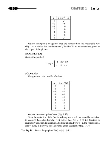
x y = x − x
−3 −24
−2 −6
−1 0
0 0
1 0
2 6
3 24

We plot these points on a pair of axes and connect them in a reasonable way
(Fig. 1.41). Notice that the domain of f is all of R, so we extend the graph to
the edges of the picture.

EXAMPLE 1.32
Sketch the graph of

−1 if x ≤ 2
f(x) =
x if x> 2

SOLUTION
We again start with a table of values.

x y = f(x)
−3 −1
−2 −1
−1 −1
0 −1
1 −1
2 −1
3 3
4 4
5 5

We plot these on a pair of axes (Fig. 1.42).
Since the definition of the function changes at x = 2, we would be mistaken
to connect these dots blindly. First notice that, for x ≤ 2, the function is
identically constant. Its graph is a horizontal line. For x> 2, the function is a
line of slope 1. Now we can sketch the graph accurately (Fig. 1.43).
√
You Try It: Sketch the graph of h(x) =|x|· 3 x.