Page 122 - Circuit Analysis II with MATLAB Applications
P. 122
Chapter 4 The Laplace Transformation
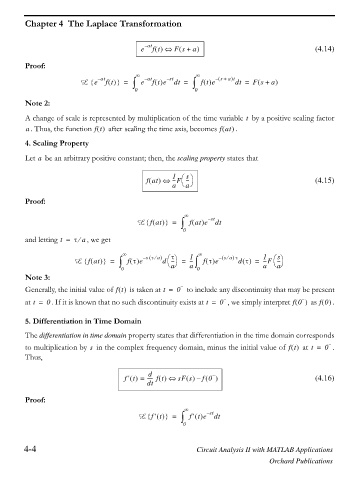
e – at ft Fs + a (4.14)
Proof:
f f
– at – at – st s + a t
–
L e ^ ft ` = ³ e ft e dt = ³ f t e dt = F s + a
0 0
Note 2:
A change of scale is represented by multiplication of the time variable by a positive scaling factor
t
a . Thus, the function f t after scaling the time axis, becomes f at .
4. Scaling Property
Let be an arbitrary positive constant; then, the scaling property states that
a
s
1 §·
-
fat --F --- (4.15)
a
a ©¹
Proof:
f
^
L fat ` = ³ fat e – st dt
0
and letting t = W a , we get
e
f W 1 f 1 s
–
e
§·
§·
-
L fat ` = ³ f W e s W a d --- = -- - ³ f W e sa W e – d W = --F -- -
^
a ©¹
a
a
a ©¹
0 0
Note 3:
Generally, the initial value of f t is taken at t = 0 to include any discontinuity that may be present
at t = 0 . If it is known that no such discontinuity exists at t = 0 , we simply interpret f 0 as f 0 .
5. Differentiation in Time Domain
The differentiation in time domain property states that differentiation in the time domain corresponds
s
to multiplication by in the complex frequency domain, minus the initial value of f t at t = 0 .
Thus,
d
f ' t = ----- ft sF s f0 – (4.16)
dt
Proof:
f
^
L f ' t ` = ³ f ' t e – st dt
0
4-4 Circuit Analysis II with MATLAB Applications
Orchard Publications

