Page 129 - Circuit Analysis II with MATLAB Applications

Properties of the Laplace Transform

T d
–
lim > sF s f0 @ = lim lim ³ ----- ft e – st dt
s o 0 s o 0 T o f H dt
H o 0
and by interchanging the limiting process, we get

T d
–
lim > sF s f0 @ = lim ³ ----- ft lim e – st dt
s o 0 T o f H dt s o 0
H o 0
Also, since
– st
lim e = 1
s o 0
the above expression reduces to

T d T
lim > sF s f0 – @ = lim ³ ----- ft dt = lim ³ f t
s o 0 T o f H dt T o f H
H o 0 H o 0
= lim > fT – f H = f f – f0
@
T o f
H o 0
and therefore,
lim sF s = f f
s o 0
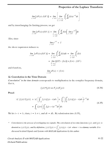
12. Convolution in the Time Domain
*
Convolution in the time domain corresponds to multiplication in the complex frequency domain,
that is,

f t *f t œ F s F s (4.34)
2
1
2
1
Proof:
f f f

L f t *f t ^ 1 2 ` = L ³ f W f t – W dW = ³ ³ f W f t – W dW e – st dt

1
2
1
2
– f 0 0
(4.35)
f f
= ³ f W ³ f t – W e – st dt dW

1
2
0 0
We let t – W = O ; then, t O= W + , and dt = dO . By substitution into (4.35),
* Convolution is the process of overlapping two signals. The convolution of two time functions f t and f t is
2
1
f
–

denoted as f t *f t , and by definition, f t *f t = ³ f W f t W dW where is a dummy variable. It is
W
1
2
2
1
2
1
– f
discussed in detail Signals and Systems with MATLAB Applications by this author.
Circuit Analysis II with MATLAB Applications 4-11
Orchard Publications