Page 125 - Classification Parameter Estimation & State Estimation An Engg Approach Using MATLAB

114 STATE ESTIMATION

. The state transition probability P t (x(i)jx(i 1)).
. The observation probability P z (z(i)jx(i)).

The expression P 0 (x(0)) with x(0) 2f1, .. . , Kg denotes the probability
that the random state variable x(0) takes the value ! x(0) . Thus
def
P 0 (k) ¼ P 0 (x(0) ¼ ! k ). Similar conventions hold for other expressions,
like P t (x(i)jx(i 1)) and P z (z(i)jx(i)).
The Markov condition of an HMM states that
P(x(i)jx(0), .. . , x(i 1)), i.e. the probability of x(i) under the condition
of all previous states, equals the transition probability. The assumption
of the validity of the Markov condition leads to a simple, yet powerful
model. Another assumption of the HMM is that the measurements are
memoryless. In other words, z(i) only depends on x(i) and not on the
states at other time points: P(z(j)jx(0), ... , x(i)) ¼ P(z(j)jx(j)).
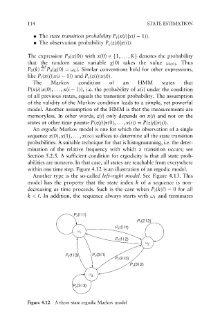
An ergodic Markov model is one for which the observation of a single
sequence x(0), x(1), .. . , x(1) suffices to determine all the state transition
probabilities. A suitable technique for that is histogramming, i.e. the deter-
mination of the relative frequency with which a transition occurs; see
Section 5.2.5. A sufficient condition for ergodicity is that all state prob-
abilities are nonzero. In that case, all states are reachable from everywhere
within one time step. Figure 4.12 is an illustration of an ergodic model.
Another type is the so-called left–right model. See Figure 4.13. This
model has the property that the state index k of a sequence is non-
decreasing as time proceeds. Such is the case when P t (kj‘) ¼ 0 for all
k <‘. In addition, the sequence always starts with ! 1 and terminates

P (1|1)
t
P (2 | 2)
t
P (2 |1)
ω t
1
P (1| 2) ω
t
2
P (1| 3) P (3|1)
t
t
P (2 | 3)
t
P (3| 2)
t
ω
3
P t (3| 3)
Figure 4.12 A three-state ergodic Markov model