Page 122 - Classification Parameter Estimation & State Estimation An Engg Approach Using MATLAB

CONTINUOUS STATE VARIABLES 111

Example 4.7 The iterated EKF for volume density estimation
In the previous example, the EKF was applied to the density estima-
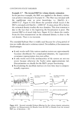
tion problem introduced in Example 4.1. The filter was initiated with
¼
the equilibrium state as prior knowledge, i.e. E[x(0)] ¼ x ¼
T
[4000 0:1] . Figure 4.11(b) shows the transient which occurs if the
T
EKF is initiated with E[x(0)] ¼ [2000 0] . It takes about 40 (s) before
the estimated density reaches the true densities. This slow transient is
due to the fact that in the beginning the linearization is poor. The
iterated EKF is of much help here. Figure 4.11(c) shows the results.
From the first measurement on the estimated density is close to the
real density. There is no transient.

The extended Kalman filter is widely used because for a long period of
time no viable alternative solution existed. Nevertheless, it has numerous
disadvantages:

. It only works well if the various random vectors are approximately
Gaussian distributed. For complicated densities, the expectation-
covariance representation does not suffice.
. It only works well if the nonlinearities of the system are not too
severe because otherwise the Taylor series approximations fail.
Discontinuities are deadly for the EKF’s proper functioning.
. Recalculating the Jacobian matrices at every time step is computa-
tionally expensive.

(a) (b) (c)
volume measurements (litre) real (thick) and estimated real (thick) and estimated
4050 volume (litre) 4020 volume (litre)
4060
4040 4010
4000 4020 4000
4000
3990
3980
3950 3980
0.1 density measurements (V) real (thick) and estimated density 0.11 real (thick) and estimated density
0.1
0.05 0.105
0.1
0 0.05
0.095
– 0.05 0 0.09
0 100 200 0 100 200 0 100 200
i∆ (s) i∆ (s) i∆ (s)
Figure 4.11 Iterated extended Kalman filtering for the volume density estimation
problem. (a) Measurements (b) Results from the EKF (c) Results from the iterated
EKF (no. of iterations ¼ 20)