Page 119 - Classification Parameter Estimation & State Estimation An Engg Approach Using MATLAB

108 STATE ESTIMATION

volume (litre) real (thin) and estimated volume (litre)
4020 4020
4000 4000
density volume error (litre)
20
0.1
0
0.09
0.08 –20
volume measurements (litre)
real (thick) and estimated density
4050
0.1
4000
0.09
3950 0.08
density measurements (V)
0.4 – 0.005 density error
0.2 0.005
0 – 0.005
i∆ (s) 0 2000 i∆ (s) 4000
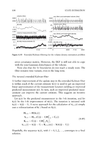
Figure 4.10 Extended Kalman filtering for the volume density estimation problem

error covariance matrix. However, the EKF is still not able to cope
with the non-Gaussian disturbances of the volume.
Note also that the 1 boundaries do not reach a steady state. The
filter remains time variant, even in the long term.

The iterated extended Kalman filter
A further improvement of the update step in the extended Kalman filter
is within reach if the current estimate x(iji) is used to get an improved
linear approximation of the measurement function yielding an improved
z
predicted measurement ^ z(i). In turn, such an improved predicted meas-
urement can improve the current estimate. This suggests an iterative
approach.
z
Let ^ z ‘ (i) be the predicted measurement in the ‘-th iteration, and let
x ‘ (i) be the ‘-th improvement of x(iji). The iteration is initiated with
x 0 (i) ¼ x(iji 1). A naive approach for the calculation of x ‘þ1 (i) simply
uses a relinearization of h( ) based on x ‘ (i).

H ‘þ1 ¼ H x ‘ ðiÞð Þ
S ‘þ1 ¼ H ‘þ1 Cðiji 1ÞH T þ C v ðiÞ
‘þ1
ð4:49Þ
K ‘þ1 ¼ Cðiji 1ÞH T S 1
‘þ1 ‘þ1
ð
ð
x ‘þ1 ðiÞ¼ xðiji 1Þþ K ‘þ1 zðiÞ h xðiji 1ÞÞÞ
Hopefully, the sequence x ‘ (i), with ‘ ¼ 0, 1, 2, .. . , converges to a final
solution.