Page 117 - Classification Parameter Estimation & State Estimation An Engg Approach Using MATLAB

106 STATE ESTIMATION

error covariance matrix C(iji). The word ‘approximate’ expresses the fact
that our estimates are not guaranteed to be unbiased due to the linear
approximations. However, we do assume that the influence of the errors
induced by the linear approximations is small. If the estimation error is
denoted by e(i), then:

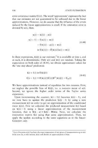
xðiÞ¼ xðijiÞ eðiÞ

ð
xði þ 1Þ¼ fxðiÞÞ þ wðiÞ
ð4:44Þ
¼ f xðijiÞ eðiÞð Þ þ wðiÞ
ffi f xðijiÞð Þ FðxðijiÞÞeðiÞþ wðiÞ

5
In these expressions, x(iji) is our estimate. It is available at time i, and
as such, it is deterministic. Only e(i) and w(i) are random. Taking the
expectation on both sides of (4.44), we obtain approximate values for
the ‘one step ahead’ prediction:

ð
xði þ 1jiÞffi f xðijiÞÞ
ð4:45Þ
T
ð
Cði þ 1jiÞffi F xðijiÞð ÞCðijiÞF xðijiÞÞ þ C w ðiÞ
We have approximations instead of equalities for two reasons. First,
we neglect the possible bias of x(iji), i.e. a nonzero mean of e(i).
Second, we ignore the higher order terms of the Taylor series
expansion.
Upon incrementing the counter, x(i þ 1ji) becomes x(iji 1), and
we now have to update the prediction x(iji 1) by using a new
measurement z(i) in order to get an approximation of the conditional
mean x(iji). First we calculate the predicted measurement ^ z(i)based
z
on x(iji 1) using a linear approximation of the measurement
x
x
function, that is h(^ x e) ffi h(^ x) H(^ x)e.Next, we calculatethe
x
innovation matrix S(i) using that same approximation. Then, we
apply the update according to the same equations as in the linear-
Gaussian case.

5
Up to this point x(iji) has been the exact expectation of x(i) given all measurements up to z(i).
From now on, in this section, x(iji) will denote an approximation of that.