Page 176 - Classification Parameter Estimation & State Estimation An Engg Approach Using MATLAB

NONPARAMETRIC LEARNING 165

T
gðyÞ¼ w y ð5:41Þ

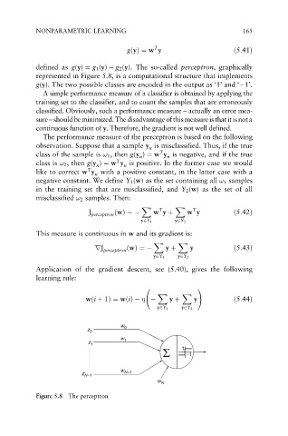
defined as g(y) ¼ g 1 (y) g 2 (y). The so-called perceptron, graphically
represented in Figure 5.8, is a computational structure that implements
g(y). The two possible classes are encoded in the output as ‘1’ and ‘ 1’.
A simple performance measure of a classifier is obtained by applying the
training set to the classifier, and to count the samples that are erroneously
classified. Obviously, such a performance measure – actually an error mea-
sure–shouldbeminimized.Thedisadvantageofthismeasureisthatitisnota
continuous function of y. Therefore, the gradient is not well defined.
The performance measure of the perceptron is based on the following
observation. Suppose that a sample y is misclassified. Thus, if the true
n
T
class of the sample is ! 1 , then g(y ) ¼ w y is negative, and if the true
n
n
T
class is ! 2 , then g(y ) ¼ w y is positive. In the former case we would
n
n
T
like to correct w y with a positive constant, in the latter case with a
n
negative constant. We define Y 1 (w) as the set containing all ! 1 samples
in the training set that are misclassified, and Y 2 (w) as the set of all
misclassified ! 2 samples. Then:
X T X T
J perceptron ðwÞ¼ w y þ w y ð5:42Þ
y2Y 1 y2Y 2
This measure is continuous in w and its gradient is:
X X
rJ perceptron ðwÞ¼ y þ y ð5:43Þ
y2Y 1 y2Y 2
Application of the gradient descent, see (5.40), gives the following
learning rule:

!
X X
wði þ 1Þ¼ wðiÞ y þ y ð5:44Þ
y2Y 1 y2Y 2

w 0
z 0
w 1
z 1
Σ 1 –1

w
z N–1 N–1
w N

Figure 5.8 The perceptron