
Page 233 - Classification Parameter Estimation & State Estimation An Engg Approach Using MATLAB
P. 233
222 UNSUPERVISED LEARNING
2. Gradient descent
(t)
. For each object y , calculate the gradient according to (7.6).
i
(t)
(t)
. Update: y (tþ1) ¼ y qE S =qy , where is a learning rate.
i
i
i
. As long as E S significantly decreases, set t ¼ t þ 1 and go to step 2.
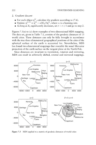
Figures 7.3(a) to (c) show examples of two-dimensional MDS mapping.
The data set, given in Table 7.1, consists of the geodesic distances of 13
world cities. These distances can only be fully brought in accordance
with the true three-dimensional geographical positions of the cities if the
spherical surface of the earth is accounted for. Nevertheless, MDS
has found two-dimensional mappings that resemble the usual Mercator
projection of the earth surface on the tangent plane at the North Pole.
Since distances are invariant to translation, rotation and mirroring,
MDS can result in arbitrarily shifted, rotated and mirrored mappings.
q =– 2 q =0
Melbourne
8000 Honolulu 8000 Honolulu
Los Angeles
4000 Tokyo 4000 Los Angeles
Melbourne Tokyo
Beijing
New York New York Beijing
0 0 Santiago
Santiago London Bangkok Bangkok
Moscow Rio London Moscow
–4000 Rio –4000
Cairo Cairo
–8000 –8000
Capetown Capetown
–8000 –4000 0 4000 8000 –8000 –4000 0 4000 8000
q =2 D =3; q =0
Melbourne
8000 Honolulu
Los Angeles
New York Honolulu
Los Angeles
4000 Santiago Tokyo
London
Tokyo London Beijing
London
Moscow
Moscow
Moscow
Beijing
0 New York Santiago
Cairo
Cairo
Rio Bangkok Rio Cairo Bangkok
London
–4000 Moscow Melbourne
Cairo
Capetown
–8000
Capetown
–8000 –4000 0 4000 8000
Figure 7.3 MDS applied to a matrix of geodesic distances of world cities