
Page 234 - Classification Parameter Estimation & State Estimation An Engg Approach Using MATLAB
P. 234
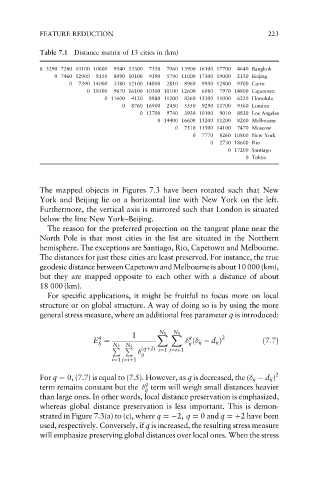
FEATURE REDUCTION                                            223

            Table 7.1 Distance matrix of 13 cities in (km)

            0 3290 7280 10100 10600  9540 13300  7350  7060 13900 16100 17700  4640 Bangkok
                0 7460 12900  8150  8090 10100  9190  5790 11000 17300 19000  2130 Beijing
                    0  7390 14000  3380 12100 14000  2810  8960  9950 12800  9500 Cairo
                         0 18500  9670 16100 10300 10100 12600  6080  7970 14800 Capetown
                             0 11600  4120  8880 11200  8260 13300 11000  6220 Honolulu
                                  0  8760 16900  2450  5550  9290 11700  9560 London
                                       0 12700  9740  3930 10100  9010  8830 Los Angeles
                                            0 14400 16600 13200 11200  8200 Melbourne
                                                0  7510 11500 14100  7470 Moscow
                                                     0  7770  8260 10800 New York
                                                          0  2730 18600 Rio
                                                               0 17200 Santiago
                                                                   0 Tokyo


            The mapped objects in Figures 7.3 have been rotated such that New
            York and Beijing lie on a horizontal line with New York on the left.
            Furthermore, the vertical axis is mirrored such that London is situated
            below the line New York–Beijing.
              The reason for the preferred projection on the tangent plane near the
            North Pole is that most cities in the list are situated in the Northern
            hemisphere. The exceptions are Santiago, Rio, Capetown and Melbourne.
            The distances for just these cities are least preserved. For instance, the true
            geodesic distance between Capetown and Melbourne is about 10 000 (km),
            but they are mapped opposite to each other with a distance of about
            18 000 (km).
              For specific applications, it might be fruitful to focus more on local
            structure or on global structure. A way of doing so is by using the more
            general stress measure, where an additional free parameter q is introduced:


                                            N S
                                                N S
                            q        1      X X     q        2
                          E ¼                        ð  ij   d ij Þ     ð7:7Þ
                            S   N  N                ij
                               P S P S
                                        ðqþ2Þ i¼1 j¼iþ1
                                       ij
                               i¼1 j¼iþ1
            For q ¼ 0, (7.7) is equal to (7.5). However, as q is decreased, the (  ij   d ij ) 2
                                        q
            term remains constant but the   term will weigh small distances heavier
                                        ij
            than large ones. In other words, local distance preservation is emphasized,
            whereas global distance preservation is less important. This is demon-
            strated in Figure 7.3(a) to (c), where q ¼ 2, q ¼ 0and q ¼þ2have been
            used, respectively. Conversely, if q is increased, the resulting stress measure
            will emphasize preserving global distances over local ones. When the stress