
Page 29 - Classification Parameter Estimation & State Estimation An Engg Approach Using MATLAB
P. 29
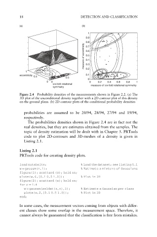
18                               DETECTION AND CLASSIFICATION

            (a)                               (b)

                                                 1
                                                0.9
                                                0.8
                                               measure of eccentricity  0.6
                                                0.7

                                                0.5
                                                0.4

                                                0.2
               1                                0.3
            eccentricity                        0.1
                   0.5
                                     0.5
                                                 0
                           0  0                   0    0.2  0.4  0.6  0.8   1
                              six-fold rotational  measure of six-fold rotational symmetry
                              symmetry
            Figure 2.4  Probability densities of the measurements shown in Figure 2.2. (a) The
            3D plot of the unconditional density together with a 2D contour plot of this density
            on the ground plane. (b) 2D contour plots of the conditional probability densities


              probabilities are assumed to be 20/94, 28/94, 27/94 and 19/94,
              respectively.
                The probabilities densities shown in Figure 2.4 are in fact not the
              real densities, but they are estimates obtained from the samples. The
              topic of density estimation will be dealt with in Chapter 5. PRTools
              code to plot 2D-contours and 3D-meshes of a density is given in
              Listing 2.1.

            Listing 2.1
            PRTools code for creating density plots.


            load nutsbolts;                  % Load the dataset; see listing 5.1
            w ¼ gaussm(z,1);                 % Estimate a mixture of Gaussians
            figure(1); scatterd (z); hold on;
            plotm(w,6,[0.1 0.5 1.0]);        % Plot in 3D
            figure(2); scatterd (z); hold on;
            for c ¼ 1: 4
              w ¼ gaussm(seldat(z,c),1);     % Estimate a Gaussian per class
              plotm(w,2,[0.1 0.5 1.0]);      % Plot in 2D
            end;

            In some cases, the measurement vectors coming from objects with differ-
            ent classes show some overlap in the measurement space. Therefore, it
            cannot always be guaranteed that the classification is free from mistakes.