
Page 31 - Classification Parameter Estimation & State Estimation An Engg Approach Using MATLAB
P. 31
20 DETECTION AND CLASSIFICATION
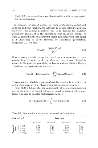
Table 2.2 is an example of a cost function that might be appropriate
for this application.
The concepts introduced above, i.e. prior probabilities, conditional
densities and cost function, are sufficient to design optimal classifiers.
However, first another probability has to be derived: the posterior
probability P(! k jz). It is the probability that an object belongs to
class ! k given that the measurement vector associated with that object
is z. According to Bayes’ theorem for conditional probabilities
(Appendix C.2) we have:
pðzj! k ÞPð! k Þ
Pð! k jzÞ¼ ð2:3Þ
pðzÞ
If an arbitrary classifier assigns a class ^ ! i to a measurement vector z
!
coming from an object with true class ! k , then a cost C(^ ! i j! k )is
!
involved. The posterior probability of having such an object is P(! k jz).
Therefore, the expectation of the cost is:
K
X
!
!
!
Rð^ ! i jzÞ¼ E½Cð^ ! i j! k Þjz¼ Cð^ ! i j! k ÞPð! k jzÞ ð2:4Þ
k¼1
This quantity is called the conditional risk. It expresses the expected cost
!
of the assignment ^ ! i to an object whose measurement vector is z.
From (2.4) it follows that the conditional risk of a decision function
^ ! !(z)is R(^ !(z)jz). The overall risk can be found by averaging the condi-
!
tional risk over all possible measurement vectors:
Z
!
!
R ¼ E½Rð^ !ðzÞjzÞ ¼ Rð^ !ðzÞjzÞpðzÞdz ð2:5Þ
z
Table 2.2 Cost function of the ‘sorting mechanical part’ application
C( ^ w i w i jw k ) in $ True class
! 1 ¼ bolt ! 2 ¼ nut ! 3 ¼ ring ! 4 ¼ scrap
0.07
0.07
Assigned class ^ ! ! ¼ bolt 0.20 0.15 0.05 0.07
0.07
^ ! ! ¼ nut
0.07
0.07
0.07
0.07
0.07
^ ! ! ¼ ring
0.03
0.03
^ ! ! ¼ scrap
0.03
0.03