Page 42 - Classification Parameter Estimation & State Estimation An Engg Approach Using MATLAB

BAYESIAN CLASSIFICATION 31

(a) (b)
1 1

0.8 0.8
measurement 2 0.6 measurement 2 0.6

0.4
0.4

0.2 0.2

0 0
0 0.2 0.4 0.6 0.8 1 0 0.2 0.4 0.6 0.8 1
measurement 1 measurement 1

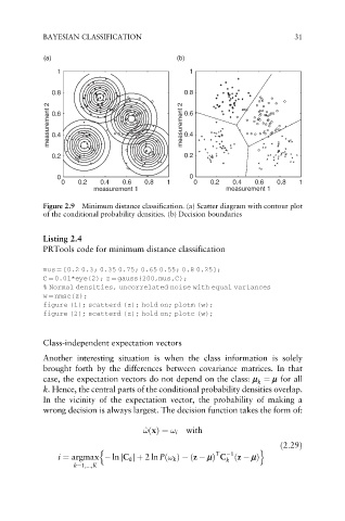
Figure 2.9 Minimum distance classification. (a) Scatter diagram with contour plot
of the conditional probability densities. (b) Decision boundaries

Listing 2.4
PRTools code for minimum distance classification

mus ¼ [0.2 0.3; 0.35 0.75; 0.65 0.55; 0.8 0.25];
C ¼ 0.01*eye(2); z ¼ gauss(200,mus,C);
% Normal densities, uncorrelated noise with equal variances
w ¼ nmsc(z);
figure (1); scatterd (z); hold on; plotm (w);
figure (2); scatterd (z); hold on; plotc (w);

Class-independent expectation vectors
Another interesting situation is when the class information is solely
brought forth by the differences between covariance matrices. In that
case, the expectation vectors do not depend on the class: m ¼ m for all
k
k. Hence, the central parts of the conditional probability densities overlap.
In the vicinity of the expectation vector, the probability of making a
wrong decision is always largest. The decision function takes the form of:

^ ! !ðxÞ¼ ! i with
ð2:29Þ
n o
T 1
i ¼ argmax ln jC k jþ 2ln Pð! k Þ ðz mÞ C ðz mÞ
k
k¼1;...;K