Page 75 - Classification Parameter Estimation & State Estimation An Engg Approach Using MATLAB

64 PARAMETER ESTIMATION

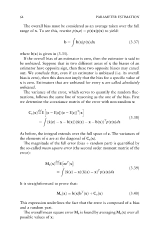
The overall bias must be considered as an average taken over the full
range of x. To see this, rewrite p(x,z) ¼ p(zjx)p(x) to yield:

Z
b ¼ bðxÞpðxÞdx ð3:37Þ

where b(x) is given in (3.35).
If the overall bias of an estimator is zero, then the estimator is said to
be unbiased. Suppose that in two different areas of x the biases of an
estimator have opposite sign, then these two opposite biases may cancel
out. We conclude that, even if an estimator is unbiased (i.e. its overall
bias is zero), then this does not imply that the bias for a specific value of
x is zero. Estimators that are unbiased for every x are called absolutely
unbiased.
The variance of the error, which serves to quantify the random fluc-
tuations, follows the same line of reasoning as the one of the bias. First
we determine the covariance matrix of the error with non-random x:

def h T i
C e ðxÞ¼E ðe E½eŠÞðe E½eŠÞ jx
Z ð3:38Þ
T
x
x
¼ ð^ xðzÞ x bðxÞÞð^ xðzÞ x bðxÞÞ pðzjxÞdz
As before, the integral extends over the full space of z. The variances of
the elements of e are at the diagonal of C e (x).
The magnitude of the full error (bias þ random part) is quantified by
the so-called mean square error (the second order moment matrix of the
error):

T
def
M e ðxÞ¼Eee jx
ð3:39Þ
Z
T
x
x
¼ ð^ xðzÞ xÞð^ xðzÞ xÞ pðzjxÞdz
It is straightforward to prove that:
T
M e ðxÞ¼ bðxÞb ðxÞþ C e ðxÞ ð3:40Þ

This expression underlines the fact that the error is composed of a bias
and a random part.
The overall mean square error M e is found by averaging M e (x) over all
possible values of x: