Page 134 - Classification Parameter Estimation & State Estimation An Engg Approach Using MATLAB

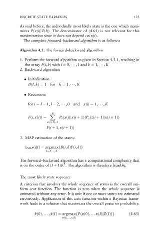
DISCRETE STATE VARIABLES 123

As said before, the individually most likely state is the one which maxi-
mizes P(x(i)jZ(I)). The denominator of (4.64) is not relevant for this
maximization since it does not depend on x(i).
The complete forward–backward algorithm is as follows:

Algorithm 4.2: The forward–backward algorithm

1. Perform the forward algorithm as given in Section 4.3.1, resulting in
the array F(i, k) with i ¼ 0, , I and k ¼ 1, , K
2. Backward algorithm:

. Initialization:
BðI; kÞ¼ 1 for k ¼ 1; ; K

. Recursion:

for i ¼ I 1, I 2, , 0 and x(i) ¼ 1, , K

K
X
Fði; xðiÞÞ ¼ P t ðxðiÞjxði þ 1ÞÞP z ðzði þ 1Þjxði þ 1ÞÞ
xðiþ1Þ¼1
Fði þ 1; xði þ 1ÞÞ

3. MAP estimation of the states:

^ x x MAP ðijIÞ¼ arg maxfBði; kÞFði; kÞg
k¼1;...; K

The forward–backward algorithm has a computational complexity that
2
is on the order of (I þ 1)K . The algorithm is therefore feasible.

The most likely state sequence
A criterion that involves the whole sequence of states is the overall uni-
form cost function. The function is zero when the whole sequence is
estimated without any error. It is unit if one or more states are estimated
erroneously. Application of this cost function within a Bayesian frame-
work leads to a solution that maximizes the overall posterior probability:

x
^ x xð0Þ; .. . ; ^ xðIÞ¼ arg maxfPðxð0Þ; .. . xðIÞjZðIÞÞg ð4:65Þ
xð0Þ;...; xðIÞ