Page 158 - Classification Parameter Estimation & State Estimation An Engg Approach Using MATLAB

PARAMETRIC LEARNING 147

w_q ¼ qdc(z,0,0.5); % Train a quadratic classifier on z
figure; scatterd(z); % Show scatter diagram of z
plotc(w_l); % Plot the first classifier
plotc(w_q,‘:’); % Plot the second classifier
[0.4 0.2] w_l labeld % Classify a new object with z ¼ [0.4 0.2]

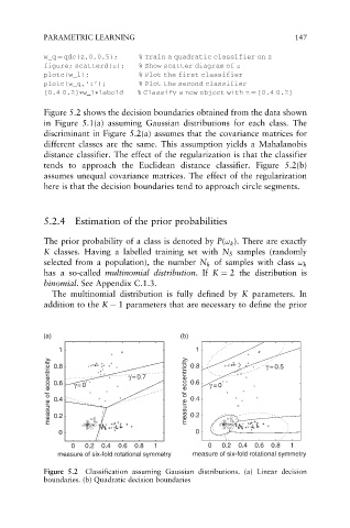
Figure 5.2 shows the decision boundaries obtained from the data shown
in Figure 5.1(a) assuming Gaussian distributions for each class. The
discriminant in Figure 5.2(a) assumes that the covariance matrices for
different classes are the same. This assumption yields a Mahalanobis
distance classifier. The effect of the regularization is that the classifier
tends to approach the Euclidean distance classifier. Figure 5.2(b)
assumes unequal covariance matrices. The effect of the regularization
here is that the decision boundaries tend to approach circle segments.

5.2.4 Estimation of the prior probabilities

The prior probability of a class is denoted by P(! k ). There are exactly
K classes. Having a labelled training set with N S samples (randomly
selected from a population), the number N k of samples with class ! k
has a so-called multinomial distribution.If K ¼ 2 the distribution is
binomial. See Appendix C.1.3.
The multinomial distribution is fully defined by K parameters. In
addition to the K 1 parameters that are necessary to define the prior

(a) (b)
1 0.8 γ = 0.5
1
measure of eccentricity 0.6 γ = 0 γ = 0.7 measure of eccentricity 0.6 γ =0
0.8

0.4
0.4
0.2

0
0 0.2
0 0.2 0.4 0.6 0.8 1 0 0.2 0.4 0.6 0.8 1
measure of six-fold rotational symmetry measure of six-fold rotational symmetry

Figure 5.2 Classification assuming Gaussian distributions. (a) Linear decision
boundaries. (b) Quadratic decision boundaries