Page 229 - Classification Parameter Estimation & State Estimation An Engg Approach Using MATLAB

218 UNSUPERVISED LEARNING

T
eigenvectors are orthogonal, this requirement is fulfilled by W N W ¼ I
N
with I the N N unit matrix. With that, W N establishes a rotation on z.
The rows of the matrix W N , i.e. the eigenvectors, must be sorted such
that the eigenvalues form a non-ascending sequence. For arbitrary D, the
matrix W D is constructed from W N by deleting the last N D rows.
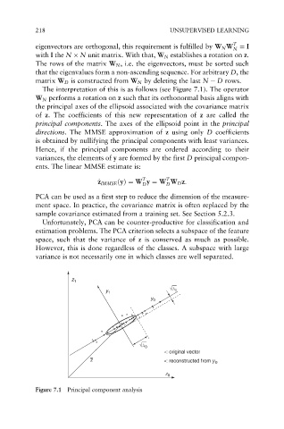
The interpretation of this is as follows (see Figure 7.1). The operator
W N performs a rotation on z such that its orthonormal basis aligns with
the principal axes of the ellipsoid associated with the covariance matrix
of z. The coefficients of this new representation of z are called the
principal components. The axes of the ellipsoid point in the principal
directions. The MMSE approximation of z using only D coefficients
is obtained by nullifying the principal components with least variances.
Hence, if the principal components are ordered according to their
variances, the elements of y are formed by the first D principal compon-
ents. The linear MMSE estimate is:

T
T
^ z lMMSE ðyÞ¼ W y ¼ W W D z:
z
D
D
PCA can be used as a first step to reduce the dimension of the measure-
ment space. In practice, the covariance matrix is often replaced by the
sample covariance estimated from a training set. See Section 5.2.3.
Unfortunately, PCA can be counter-productive for classification and
estimation problems. The PCA criterion selects a subspace of the feature
space, such that the variance of z is conserved as much as possible.
However, this is done regardless of the classes. A subspace with large
variance is not necessarily one in which classes are well separated.

z 1
√λ 1
y 1
y 0

√λ 0
: original vector
z : reconstructed from y 0

z 0
Figure 7.1 Principal component analysis