Page 250 - Classification Parameter Estimation & State Estimation An Engg Approach Using MATLAB

CLUSTERING 239

3. Maximization step (M step): Optimize the model parameters
^
m
C (iþ1) ¼f^ k , ^ m , C k g by maximum likelihood estimation using the
C

k
expectation x n calculated in the previous step. See (7.27) and (7.28).
x
4. Stop if the likelihood did not change significantly in step 3. Else,
increment i and go to step 2.
Clustering by EM results in more flexible cluster shapes than K-means
clustering. It is also guaranteed to converge to (at least) a local optimum.
However, it still has some of the same problems of K-means: the choice
of the appropriate number of clusters, the dependence on initial condi-
tions and the danger of convergence to local optima.

Example 7.3 Classification of mechanical parts, EM algorithm for
mixture of Gaussians
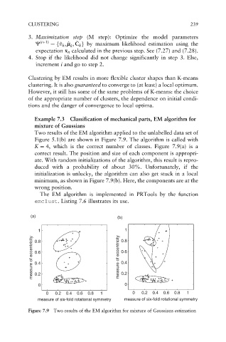
Two results of the EM algorithm applied to the unlabelled data set of
Figure 5.1(b) are shown in Figure 7.9. The algorithm is called with
K ¼ 4, which is the correct number of classes. Figure 7.9(a) is a
correct result. The position and size of each component is appropri-
ate. With random initializations of the algorithm, this result is repro-
duced with a probability of about 30%. Unfortunately, if the
initialization is unlucky, the algorithm can also get stuck in a local
minimum, as shown in Figure 7.9(b). Here, the components are at the
wrong position.
The EM algorithm is implemented in PRTools by the function
emclust. Listing 7.6 illustrates its use.

(a) (b)

1
1 0.8
measure of eccentricity 0.6 measure of eccentricity 0.6
0.8

0.4
0.4
0.2

0
0 0.2
0 0.2 0.4 0.6 0.8 1 0 0.2 0.4 0.6 0.8 1
measure of six-fold rotational symmetry measure of six-fold rotational symmetry

Figure 7.9 Two results of the EM algorithm for mixture of Gaussians estimation