Page 76 - Classification Parameter Estimation & State Estimation An Engg Approach Using MATLAB
P. 76
PERFORMANCE OF ESTIMATORS 65
Z
def
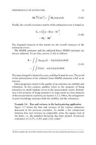
M e ¼E ee T ¼ M e ðxÞpðxÞdx ð3:41Þ
Finally, the overall covariance matrix of the estimation error is found as:
h i
T
C e ¼ E ðe bÞðe bÞ
ð3:42Þ
¼ M e bb T
The diagonal elements of this matrix are the overall variances of the
estimation errors.
The MMSE estimator and the unbiased linear MMSE estimator are
always unbiased. To see this, rewrite (3.36) as follows:
ZZ
x
b ¼ ð^ x MMSE ðzÞ xÞpðxjzÞpðzÞdxdz
ð3:43Þ
ZZ
¼ ðE½xjz xÞpðxjzÞpðzÞdxdz
The inner integral is identical to zero, and thus b must be zero. The proof
of the unbiasedness of the unbiased linear MMSE estimator is left as an
exercise.
Other properties related to the quality of an estimator are stability and
robustness. In this context, stability refers to the property of being
insensitive to small random errors in the measurement vector. Robust-
ness is the property of being insensitive to large errors in a few elements
of the measurements (outliers); see Section 3.3.2. Often, the enlargement
of prior knowledge increases both the stability and the robustness.
Example 3.6 Bias and variance in the backscattering application
Figure 3.7 shows the bias and variance of the various estimators
discussed in the previous examples. To enable a fair comparison
between bias and variance in comparable units, the square root of
the latter, i.e. the standard deviation, has been plotted. Numerical
evaluation of (3.37), (3.41) and (3.42) yields: 3
3
In this example, the vector b(x) and the matrix C(x) turn into scalars because here x is a scalar.

