Page 119 - Compact Numerical Methods For Computers

108 Compact numerical methods for computers
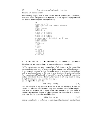
Example 9.1. Inverse iteration

The following output, from a Data General NOVA operating in 23-bit binary
arithmetic, shows the application of algorithm 10 to the algebraic eigenproblem of
the order-4 Hilbert segment (see appendix 1).

RUN
ENHGII OCT 21 76
GAUSS ELIMINATION FOR INVERSE: ITERATION
ORDER=? 4
HILBERT SEGMENT
SHIFT=? 0
APPROX EV= 0
APPROX EV= 9.67397E-5
APPROX EV= 9.66973E-5
APPROX EV= 9.66948E-5
APPROX EV= 9.66948E-5
CONVERGED TO EV= 9.66948E-5 IN 5 ITNS
4 EQUAL CPNTS
HILBERT SEGMENT
VECTOR
-2.91938E-2
.328714
-.791412
.514551
RESIDUALS
-2.98023E-8
-7.45058E-8
-2.98023E-8
-2.98023E-8

9.3. SOME NOTES ON THE BEHAVIOUR OF INVERSE ITERATION
The algorithm just presented may in some details appear complicated.
(i) The convergence test uses a comparison of all elements in the vector. For
many applications the norm of y or some similar measure may suffice; however, it
is not foolproof, particularly when the starting vector is set to some simple choice
such as a column of ones. In this case, inverse iteration with a diagonal matrix
A = i, a unit matrix B and a shift of zero will ‘converge’ at iteration 2, which is its
ii
earliest opportunity to stop. However, the vector is left very much in error,
though the dominant component has converged.
(ii) The eigenvalue is given by
shift + x / y = k + x / y (9.20)
i i i i
from the analysis of equations (9.16)-(9.18). When the element y i is zero, of
course, this is not suitable for determining the eigenvalue. Therefore the program
must save the vectors x and y, search for the largest element in y, then divide it
into the corresponding element of x in order to get the eigenvalue. It is tempting
to suggest that the expression should be simply
shift + 1/y = k + 1/y i (9.21)
i
since a normalisation is performed at each stage. Alas, too many matrices have