Page 123 - Compact Numerical Methods For Computers

112 Compact numerical methods for computers
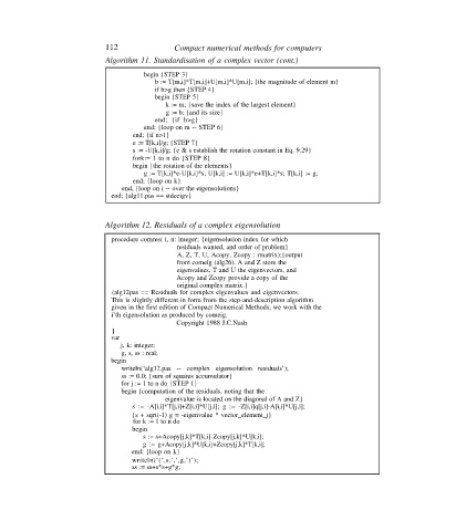
Algorithm 11. Standardisation of a complex vector (cont.)

begin {STEP 3}
b := T[m,i]*T[m,i]+U[m,i]*U[m,i]; {the magnitude of element m}
if b>g then {STEP 4}
begin {STEP 5}
k := m; {save the index of the largest element}
g := b; {and its size}
end; {if b>g}
end; {loop on m -- STEP 6}
end; {if n>1}
e := T[k,i]/g; {STEP 7}
s := -U[k,i]/g; {e & s establish the rotation constant in Eq. 9.29}
fork:= 1 to n do {STEP 8}
begin {the rotation of the elements}
g := T[k,i]*e-U[k,i]*s; U[k,i] := U[k,i]*e+T[k,i]*s; T[k,i] := g;
end; {loop on k}
end, {loop on i -- over the eigensolutions}
end; {alg11.pas == stdceigv}

Algorithm 12. Residuals of a complex eigensolution

procedure comres( i, n: integer; {eigensolution index for which
residuals wanted, and order of problem}
A, Z, T, U, Acopy, Zcopy : rmatrix);{output
from comeig (alg26). A and Z store the
eigenvalues, T and U the eigenvectors, and
Acopy and Zcopy provide a copy of the
original complex matrix.}
(alg12pas == Residuals for complex eigenvalues and eigenvectors.
This is slightly different in form from the step-and-description algorithm
given in the first edition of Compact Numerical Methods; we work with the
i’th eigensolution as produced by comeig.
Copyright 1988 J.C.Nash
}
var
j, k: integer;
g, s, ss : real;
begin
writeln(‘alg12.pas -- complex eigensolution residuals’);
ss := 0.0; {sum of squares accumulator}
for j := 1 to n do {STEP 1}
begin {computation of the residuals, noting that the
eigenvalue is located on the diagonal of A and Z}
s := -A[i,i]*T[j,i]+Z[i,i]*U[j,i]; g := -Z[i,i]q[j,i]-A[i,i]*U[j,i];
{s + sqrt(-1) g = -eigenvalue * vector_element_j}
for k := 1 to n do
begin
s := s+Acopy[j,k]*T[k,i]-Zcopy[j,k]*U[k,i];
g := g+Acopy[j,k]*U[k,i]+Zcopy[j,k]*T[k,i];
end; {loop on k}
writeln(‘(‘,s,’,‘,g,’)’);
ss := ss+s*s+g*g;