Page 142 - Compact Numerical Methods For Computers

Real symmetric matrices 131
Example 10.2. Application of the Jacobi algorithm in celestial mechanics
It is appropriate to illustrate the use of algorithm 14 by Jacobi’s (1846) own
example. This arises in the study of orbital perturbations of the planets to
compute corrections to some of the parameters of the solar system. Unfortunately
at the time Jacobi was writing his paper, Neptune had not been discovered.
Leverrier reported calculations suggesting the existence of this planet on 31
August 1846, to l’Académie des Sciences in Paris, and Galle in Berlin confirmed
this hypothesis by observation less than three weeks later on 18 September. The
derivation of the eigenproblem in this particular case is lengthy and irrelevant to
the present illustration, so we will begin with Jacobi’s equations V. These give a
non-symmetric matrix à which can be symmetrised by a diagonal transformation
resulting in Jacobi’s equations VIII, where the off-diagonal elements are expres-
sed in terms of their common logarithms to which 10 has been added. I decided to
work with the non-symmetric form and symmetrised it by means of
½
A ij = A ji = (Ã Ã ) .
ji
ij
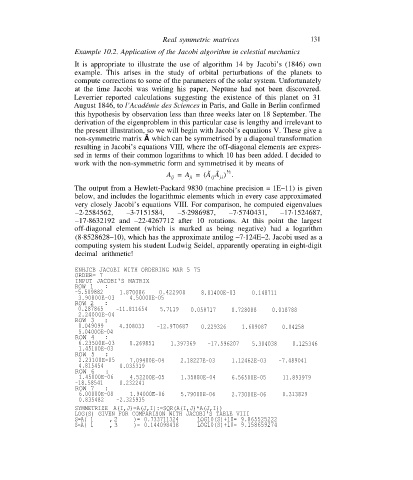
The output from a Hewlett-Packard 9830 (machine precision = 1E–11) is given
below, and includes the logarithmic elements which in every case approximated
very closely Jacobi’s equations VIII. For comparison, he computed eigenvalues
–2·2584562, –3·7151584, –5·2986987, –7·5740431, –17·1524687,
–17·8632192 and –22·4267712 after 10 rotations. At this point the largest
off-diagonal element (which is marked as being negative) had a logarithm
(8·8528628–10), which has the approximate antilog –7·124E–2. Jacobi used as a
computing system his student Ludwig Seidel, apparently operating in eight-digit
decimal arithmetic!

ENHJCB JACOBI WITH ORDERING MAR 5 75
ORDER= 7
INPUT JACOBI'S MATRIX
ROW 1 :
-5.509882 1.870086 0.422908 8.81400E-03 0.148711
3.90800E-03 4.50000E-05
ROW 2 :
0.287865 -11.811654 5.7119 0.058717 0.728088 0.018788
2.24000E-04
ROW 3 :
0.049099 4.308033 -12.970687 0.229326 1.689087 0.04258
5.04OOOE-04
ROW 4 :
6.23500E-03 0.269851 1.397369 -17.596207 5.304038 0.125346
1.45100E-03
ROW 5 :
2.23100E-05 7.09480E-04 2.18227E-03 l.l2462E-03 -7.489041
4.815454 0.035319
ROW 6 :
1.45000E-06 4.52200E-05 1.35880E-04 6.56500E-05 11.893979
-18.58541 0.232241
ROW 7 :
6.00000E-08 1.94000E-06 5.79000E-06 2.73000E-06 0.313829
0.835482 -2.325935
SYMMETRIZE A(I,J)=A(J,I):=SQR(A(I,J)*A(J,I))
LOG(S) GIVEN FOR COMPARISON WITH JACOBI'S TABLE VIII
S=A( 1 ,2 )= 0.733711324 LOG10(S)+l0= 9.865525222
S=A( 1 ,3 )= 0.144098438 LOG10(S)+l0= 9.158659274