Page 144 - Compact Numerical Methods For Computers

Real symmetric matrices 133
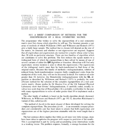
EIGENVALUE 6 =-17.86329687 VECTOR:
0.016712951 -0.363977437 0.462076406 -0.808519448 6.627116-04
4.72676E-03 -1.36341E-04
EIGENVALUE 7 =-22.42730849 VECTOR:
3.56838E-05 -3.42339E-04 2.46894E-03 6.41285E-03 -0.451791590
0.891931555 -0.017179128
MAXIMUM ABSOLUTE RESIDUAL= 9.51794E-10
MAXIMUM ABSOLUTE INNER PRODUCT= 1.11326E-11

10.5. A BRIEF COMPARISON OF METHODS FOR THE
EIGENPROBLEM OF A REAL SYMMETRIC MATRIX

The programmer who wishes to solve the eigenproblem of a real symmetric
matrix must first choose which algorithm he will use. The literature presents a vast
array of methods of which Wilkinson (1965) and Wilkinson and Reinsch (1971)
give a fairly large sample. The method that is chosen will depend on the size of
the matrix, its structure and whether or not eigenvectors are required. Suppose
that all eigenvalues and eigenvectors are wanted for a matrix whose order is less
than 20 with no particular structure. There are two families of algorithm which
are candidates to solve this problem. The first reduces the square matrix to a
tridiagonal form of which the eigenproblem is then solved by means of one of
several variants of either the QR algorithm or bisection. (Bisection will find only
eigenvalues; inverse iteration is used to obtain the eigenvectors.) The eigenvectors
of the tridiagonal matrix must then be back-transformed to find those of the
original matrix. Because this family of methods—tridiagonalisation, solution of
reduced form, back-transformation—requires fairly complicated codes from the
standpoint of this work, they will not be discussed in detail. For matrices of order
greater than 10, however, the Householder tridiagonalisation with the QL al-
gorithm as described by Wilkinson and Reinsch (1971) is probably the most
efficient method for the solution of the complete eigenproblem of a real sym-
metric matrix. (Some studies by Dr Maurice Cox of the UK National Physical
Laboratory show that Givens’ tridiagonalisation, if carefully coded, usually in-
volves less work than that of Householder.) It is probably worthwhile for the user
with many eigenproblems to solve of order greater than 10 to implement such a
method.
The other family of methods is based on the Jacobi algorithm already discussed.
Wilkinson, in Wilkinson and Reinsch (1971, pp 192-3), describes Rutishauser’s

variant of this, called jacobi:
‘The method of Jacobi is the most elegant of those developed for solving the
complete eigenproblem. The procedure jacobi. . . is an extremely compact proce-
dure and considerable care has been taken to ensure that both eigenvalues and
eigenvectors are of the highest precision attainable with the word length that is
used.’
The last sentence above implies that while jacobi uses very little storage, steps
have been taken to optimise the program with respect to precision of the results.
This is accomplished in part by saving and accumulating some intermediate results
in a working vector. The problem requires, formally, n storage locations for the