Page 149 - Compact Numerical Methods For Computers

138 Compact numerical methods for computers
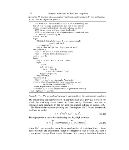
Algorithm 15. Solution of a generalised matrix eigenvalue problem by two applications
of the Jacobi algorithm (cont.)
{**** WARNING **** No check is made to see that the sweep limit
has not been exceeded. Cautious users may wish to pass back the
number of sweeps and the limit value and perform a test here.}
{STEP 3 is not needed in this version of the algorithm.}
{STEP 4 -- transformation of initial eigenvectors and creation of matrix
C, which we store in array B}
for i := 1 to n do
begin
if B[i,i]c=0.0 then halt; {matrix B is not computationally
positive definite.}
s := 1.0/sqrt(B[i,i]);
for j := 1 to n do V[j,i] := s * V[j,i]; {to form Bihalf}
end; {loop on i}
{STEP 5 -- not needed as matrix A already entered}
{STEP 6 -- perform the transformation 11.11b}
for i := l to n do
begin
for j := i to n do {NOTE: i to n NOT 1 to n}
begin
s := 0.0;
for k := 1 to n do
for m := 1 to n do
s := s+V[k,i]*A[k,m]*V[m,j];
B[i.j] := s; B[j,i] := s;
end; {loop on j}
end; {loop on i}
{STEP 7 -- revised to provide simpler Pascal code}
initev := false; {Do not initialize eigenvectors, since we have
provided the initialization in STEP 4.}
writeln(‘Eigensolutions of general problem’);
evJacobi(n, B, V, initev); {eigensolutions of generalized problem}
end; {alg15.pas == genevJac}

Example 11.1. The generalised symmetric eigenproblem: the anharmonic oscillator
The anharmonic oscillator problem in quantum mechanics provides a system for
which the stationary states cannot be found exactly. However, they can be
computed quite accurately by the Rayleigh-Ritz method outlined in example 2.5.
The Hamiltonian operator (Newing and Cunningham 1967) for the anharmonic
oscillator is written
2 2 2 4
H = –d /dx + k x + k x . (11.22)
2
4
The eigenproblem arises by minimising the Rayleigh quotient
(11.23)

where f(x ) is expressed as some linear combination of basis functions. If these
basis functions are orthonormal under the integration over the real line, then a
conventional eigenproblem results; However, it is common that these functions