Page 177 - Compact Numerical Methods For Computers

166 Compact numerical methods for computers

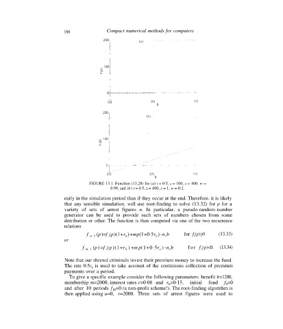
FIGURE 13.1. Function (13.28) for (a) t = 0·5, z = 100, s = 100. w =
0·99, and (b) t = 0·5, z = 100, s = 1, w = 0·2.

early in the simulation period than if they occur at the end. Therefore. it is likely
that any sensible simulation. will use root-finding to solve (13.32) for p for a
variety of sets of arrest figures n. In particular, a pseudo-random-number
generator can be used to provide such sets of numbers chosen from some
distribution or other. The function is then computed via one of the two recurrence
relations

f i+ 1 (p)=f (p)(1+r )+mp(1+0·5r )-n b for f (p)>0 (13.33)
i
e
i
i
e
or
f i+ 1 (p) =f (p)(1+r ) +m p(1+0·5r ) -n b f o r f (p)<0. (13.34)
i
b
e
i
i
Note that our shrewd criminals invest their premium money to increase the fund.
The rate 0·5r e is used to take account of the continuous collection of premium
payments over a period.
To give a specific example consider the following parameters: benefit b=1200,
membership m=2000, interest rates r=0·08 and r =0·15, initial fund f =0
0
b
and after 10 periods f =0 (a non-profit scheme!). The root-finding algorithm is
10
then applied using u=0, v=2000. Three sets of arrest figures were used to