Page 215 - Compact Numerical Methods For Computers

204 Compact numerical methods for computers

Algorithm 22. Function minimisation by conjugate gradients (cont.)
if oldstep>1.0 then oldstep:=1.0; {with a limitation to prevent too
large a step being taken. This strategy follows Nash &
Walker-Smith in multiplying the best step by 1.7 and then
limiting the resulting step to length = 1}
until (count=n) or (G1<=tol) or (cycle=cyclimit);
{this ends the cg cycle loop}
until (cycle=l) and ((count=n) or (G1<=tol));
{this is the convergence condition to end loop at STEP 2}
end; {begin minimisation}
writeln(‘Exiting from Alg22.pas conjugate gradients minimiser’);
writeln(‘ ’, funcount, ’ function evaluations used’);
writeln(‘ ’, gradcount, ’ gradient evaluations used’);
end; {alg22.pas == cgmin}

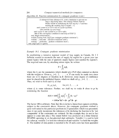
Example 16.1. Conjugate gradients minimisation
In establishing a tentative regional model of hog supply in Canada, Dr J J
Jaffrelot wanted to reconcile the sum of supply by region for a given year (an
annual figure) with the sum of quarterly supply figures (not reported by regions!).
The required sum can, by attaching minus signs, be written

where the b are the parameters which should give T=0 when summed as shown
j
with the weights w. Given w , j=1, 2, . . . , n, T can easily be made zero since
j
there are (n-1) degrees of freedom in b. However, some degree of confidence
must be placed in the published figures, which we shall call p , j=1, 2, . . . , n.
j
Thus, we wish to limit each b so that
j
| b -p |<d j for j=1, 2, . . . , n
j
j
where d j is some tolerance. Further, we shall try to make b close to p by
minimising the function

The factor 100 is arbitrary. Note that this is in fact a linear least-squares problem,
subject to the constraints above. However, the conjugate gradients method is
quite well suited to the particular problem in 23 parameters which was presented,
since it can easily incorporate the tolerances d by declaring the function to be ‘not
j
computable’ if the constraints are violated. (In this example they do not in fact
appear to come into play.) The output below was produced on a Data General
ECLIPSE operating in six hexadecimal digit arithmetic. Variable 1 is used to hold
the values p, variable 2 to hold the tolerances d and variable 3 to hold the weights
w. The number of data points is reported to be 24 and a zero has been appended