Page 227 - Compact Numerical Methods For Computers

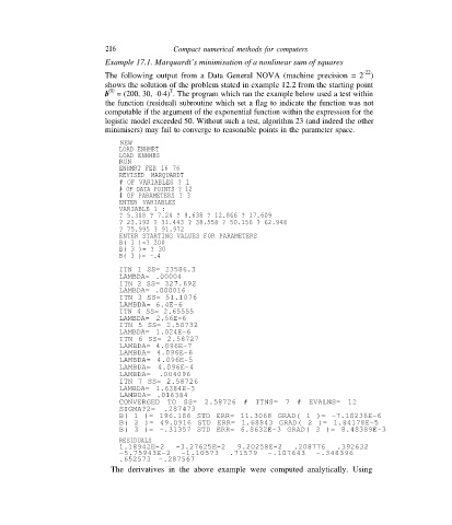
216 Compact numerical methods for computers
Example 17.1. Marquardt’s minimisation of a nonlinear sum of squares
-22
The following output from a Data General NOVA (machine precision = 2 )
shows the solution of the problem stated in example 12.2 from the starting point
(0) T
b = (200, 30, -0·4) . The program which ran the example below used a test within
the function (residual) subroutine which set a flag to indicate the function was not
computable if the argument of the exponential function within the expression for the
logistic model exceeded 50. Without such a test, algorithm 23 (and indeed the other
minimisers) may fail to converge to reasonable points in the parameter space.
NEW
LOAD ENHMRT
LOAD ENHHBS
RUN
ENHMRT FEB 16 76
REVISED MARQUARDT
# OF VARIABLES ? 1
# OF DATA POINTS ? 12
# OF PARAMETERS ? 3
ENTER VARIABLES
VARIABLE 1 :
? 5.308 ? 7.24 ? 9.638 ? 12.866 ? 17.609
? 23.192 ? 31.443 ? 38.558 ? 50.156 ? 62.948
? 75.995 ? 91.972
ENTER STARTING VALUES FOR PARAMETERS
B( 1 )=? 200
B( 3 )= ? 30
B( 3 )= -.4
ITN 1 SS= 23586.3
LAMBDA= .00004
ITN 2 SS= 327.692
LAMBDA= .000016
ITN 3 SS= 51.1076
LAMBDA= 6.4E-6
ITN 4 SS= 2.65555
LAMBDA= 2.56E-6
ITN 5 SS= 2.58732
LAMBDA= 1.024E-6
ITN 6 SS= 2.58727
LAMBDA= 4.096E-7
LAMBDA= 4.096E-6
LAMBDA= 4.096E-5
LAMBDA= 4.096E-4
LAMBDA= .004096
ITN 7 SS= 2.58726
LAMBDA= 1.6384E-3
LAMBDA= .016384
CONVERGED TO SS= 2.58726 # ITNS= 7 # EVALNS= 12
SIGMA?2= .287473
B( 1 )= 196.186 STD ERR= 11.3068 GRAD( 1 )= -7.18236E-6
B( 2 )= 49.0916 STD ERR= 1.68843 GRAD( 2 )= 1.84178E-5
B( 3 )= -.31357 STD ERR= 6.8632E-3 GRAD( 3 )= 8.48389E-3
RESIDUALS
1.18942E-2 -3.27625E-2 9.20258E-2 .208776 .392632
-5.75943E-2 -1.10573 .71579 -.107643 -.348396
.652573 -.287567
The derivatives in the above example were computed analytically. Using