
Page 242 - Compact Numerical Methods For Computers
P. 242
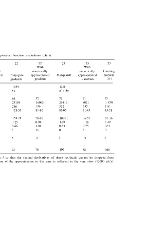
TABLE  18.5. Comparison of algorithm performance as measured by equivalent function evaluations (efe’s).

 Algorithm  19+20  21  21  22  22    23            23           23
 With                  With                       With
 numerically        numerically                numerically   Omitting
 Type  Nelder–  Variable  approximated  Conjugate  approximated  Marquardt  approximated  problem
 Mead  metric  gradient  gradients  gradient     Jacobian       34†

 Code length†  1242  1068  1059     1231
                                     2
 2
 2
 Array elements  n  + 4n + 2  n  + 5n  5n  n  + 5n
 (a) number of
 successful runs  68  68  51  66  52  76         61           75
 (b) total efe’s  33394  18292  10797  29158  16065  26419  8021  1 4399
 (c) total parameters  230  261  184  236  196  322  255      318
 (d) w 1  = (b)/(c)  145·19  70·08  58·68  123·55  81·96  82·05  31·45  45·28
 (e) w 0  = average efe’s
 per parameter  141·97  76·72  88·25  154·78  78·96  106·01  36·57  67·36
 0·98  1·09  1·50  1·25  0·96       1·29          1·16        1·49
 (f) r = w 0 /W l
 (g) a = 1/(2r – 1)  105  0·84  0·50  0·66  1·08  0·63  0·75  0·51
 (h) number of failures  6  3  20  5  16  0      8            0
 (i) number of problems
 not run  5  8  8  8  11            3             10          4
 (j) successes as
 percentage of
 problems run  92  96  72  93  76   100          88           100

 † Problem 34 of the set of 79 has been designed to have residuals f so that the second derivatives of these residuals cannot be dropped from
 equation ( 17, 15) to make the Gauss–Newton approximation. The failure of the approximation in this case is reflected in the very slow (12000 efe’s)
 convergence of algorithm 23.
 ‡ On Data General NOVA (23-bit mantissa).