Page 252 - Compact Numerical Methods For Computers

Conjugate gradients method in linear algebra 239
matrix is not definite, the normal equations

A Ax=A b (19.13)
T
T
provide a non-negative definite matrix A A. Finally, the problem can be ap-
T
proached in a completely different way. Equation (2.13) can be rewritten
3 2 2 2
y j+ l =7jh +[2-h /(1+j h ) ]y -y j- 1 . (19.14)
j
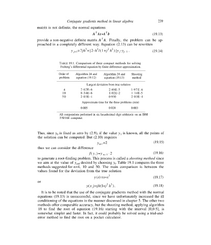
TABLE 19.1. Comparison of three compact methods for solving
Froberg’s differential equation by finite difference approximation.

Order of Algorithm 24 and Algorithm 24 and Shooting
problem equation (19.12) equation (19.13) method

Largest deviation from true solution
4 2·62E-6 2·88E-5 l·97E-6
10 8·34E-6 1·02E-2 1·14E-5
50 2·03E-4 0·930 2·03E-4
Approximate time for the three problems (min)
0·005 0·028 0·003
All computations performed in six hexadecimal digit arithmetic on an IBM
370/168 computer.

Thus, since y is fixed as zero by (2.9), if the value y is known, all the points of
0 1
the solution can be computed. But (2.10) requires
y n+1 =2 (19.15)
thus we can consider the difference
f( y ) =y n+ 1 - 2 (19.16)
1
to generate a root-finding problem. This process is called a shooting method since
we aim at the value of y desired by choosing y . Table 19.1 compares the three
l
n+l
methods suggested for n=4, 10 and 50. The main comparison is between the
values found for the deviation from the true solution
3
y (x) =x+x (19.17)
or
2 2
y(x )=jh(l+j h ). (19.18)
j
It is to be noted that the use of the conjugate gradients method with the normal
equations (19.13) is unsuccessful, since we have unfortunately increased the ill
conditioning of the equations in the manner discussed in chapter 5. The other two
methods offer comparable accuracy, but the shooting method, applying algorithm
18 to find the root of equation (19.16) starting with the interval [0,0·5], is
somewhat simpler and faster. In fact, it could probably be solved using a trial-and-
error method to find the root on a pocket calculator.