Page 256 - Compact Numerical Methods For Computers

Conjugate gradients method in linear algebra 243
to be used to compute the eigenvalue approximation
(19.25)

where b is the largest element in magnitude in b (but keeps its sign!!), I use the
m
infinity norm (9.14) in computing the next iterate x from b. To obtain an
eigenvector normalised so that
T
x Bx=1 (19.26)
one has only to form
T T
x c =x Bx . (19.27)
At the point where the norm of r is compared to the tolerance to determine if the
algorithm has converged, c is once again available from the computation (19.21).
T
The residual norm ||r|| should be divided by (x Bx)½ if x is normalised by this
quantity.
Since only the solution procedure for the linear equations arising in inverse
iteration has been changed from algorithm 10 (apart from the convergence
criterion), the method outlined in the above suggestions will not converge any
faster than a more conventional approach to inverse iteration. Indeed for prob-
lems which are ill conditioned with respect to solution via the conjugate gradients
algorithm 24, which nominally requires that the coefficient matrix H be non-
negative definite, the present method may take many more iterations. Neverthe-
less, despite the handicap that the shift s cannot be too close to the eigenvalue or
the solution vector b will ‘blow up’, thereby upsetting the conjugate gradients
process, inverse iteration performed in the manner described does provide a tool
for finding or improving eigensolutions of large matrices on a small computer.
Examples are given at the end of §19.4.

19.4. EIGENSOLUTIONS BY MINIMISING THE RAYLEIGH
QUOTIENT

Consider two symmetric matrices A and B where B is also positive definite. The
Rayleigh quotient defined by
T T
R=x Ax/x Bx (19.28)
then takes on its stationary values (that is, the values at which the partial
derivatives with respect to the components of x are zero) at the eigensolutions of
Ax=eBx. (2.63)
In particular, the maximum and minimum values of R are the extreme eigen-
values of the problem (2.63). This is easily seen by expanding

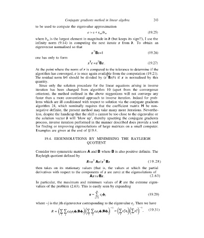
(19.29)

where ~j is the jth eigenvector corresponding to the eigenvalue e . Then we have
j
(19.31)