Page 48 - Compact Numerical Methods For Computers
P. 48
38                Compact numerical methods for computers
                            Algorithm 1. Singular-value decomposition (cont.)

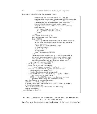
                                           current sweep. That is, we now go to STEP 11. The first
                                           condition checks for very small column norms in BOTH columns, for
                                           which no rotation makes sense. The second condition determines
                                           if the inner product is small with respect to the larger of the
                                           columns, which implies a very small rotation angle.)
                                           else {columns are in order, but their inner product is not small}
                                           begin {STEP 8}
                                              p := p/q; r := 1-r/q; vt := sqrt(4*p*p + r*r);
                                              c0 := sqrt(0.5*(1+r/vt)); s0 := p/(vt*c0);
                                              rotate;
                                           end
                                        end {columns in order with q>=r}
                                        else {columns out of order -- must rotate}
                                         begin {STEP 9}
                                            {note: r > q, and cannot be zero since both are sums of squares for
                                           the svd. In the case of a real symmetric matrix, this assumption
                                           must be questioned.}
                                           p := p/r; q := q/r-1; vt := sqrt(4*p*p + q*q);
                                           s0 := sqrt(0.5*(1-q/vt));
                                           if p<0 then s0 := -s0;
                                           co := p/(vt*s0);
                                           rotate; {The rotation is STEP 10.}
                                         end;
                                         {Both angle calculations have been set up so that large numbers do
                                        not occur in intermediate quantities. This is easy in the svd case,
                                         since quantities x2,y2 cannot be negative. An obvious scaling for
                                         the eigenvalue problem does not immediately suggest itself.)
                                      end; {loop on K -- end-loop is STEP 11}
                                   end; {loop on j -- end-loop is STEP 12}
                                   writeln(‘End of Sweep #’, SweepCount,
                                         ‘- no. of rotations performed =’, RotCount);
                                   {STEP 13 -- Set EstColRank to largest column index for which
                                      Z[column index] > (Z[1]*tol + tol*tol)
                                      Note how Pascal expresses this more precisely.}
                                   while (EstColRank >= 3) and (Z[EstColRank] <= Z[1]*tol + tol*tol)
                                         do EstColRank := EstColRank-1;
                                      {STEP 14 -- Goto STEP 1 to repeat sweep if rotations have been
                                         performed and the sweep limit has not been reached.}
                                until (RotCount=0) or (SweepCount>slimit);
                                {STEP 15 -- end SVD calculations}
                                if (SweepCount > slimit) then writeln(‘**** SWEEP LIMIT EXCEEDED’);
                                if (SweepCount > slimit) then
                                {Note: the decomposition may still be useful, even if the sweep
                                limit has been reached.}
                             end; {alg01.pas == NashSVD}


                             3.5. AN ALTERNATIVE IMPLEMENTATION OF THE SINGULAR-
                                                  VALUE DECOMPOSITION
                           One of the most time-consuming steps in algorithm 1 is the loop which comprises

