
Page 52 - Compact Numerical Methods For Computers
P. 52
42 Compact numerical methods for computers
residual sum of squares. However, if a component with a very small singular value
is introduced, it will contribute a very large amount to the corresponding element
of w, and x will acquire large elements also. From (3.48), however, it is the
interaction between the normalised component u j and b which determines how
much a given component reduces the sum of squares. A least-squares problem
will therefore be ill conditioned if b is best approximated by a column of U which
is associated with a small singular value and thus may be computed inaccurately.
On the other hand, if the components corresponding to ‘large’ singular values
are the ones which are responsible for reducing the sum of squares, then the
problem has a solution which can be safely computed by leaving out the
components which make the elements of w and x large without appreciably
reducing the sum of squares. Unless the unwanted components have no part in
reducing the sum of squares, that is unless
u i T b = 0 for i > k (3.49)
under the same condition (3.46) for k, then solutions which omit these components
are not properly termed least-squares solutions but principal-components solutions.
In many least-squares problems, poorly determined components will not arise,
all singular values being of approximately the same magnitude. As a rule of
thumb for my clients, I suggest they look very carefully at their data, and in
particular the matrix A, if the ratio of the largest singular value to the smallest
exceeds 1000. Such a distribution of singular values suggests that the columns of A
are not truly independent and, regardless of the conditioning of the problem as
discussed above, one may wish to redefine the problem by leaving out certain
variables (columns of A) from the set used to approximate b.
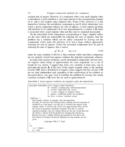
Algorithm 2. Least-squares solution via singular-value decomposition
procedure svdlss(nRow, nCo1: integer; {order of problem}
W : wmatrix; {working array with decomposition}
Y : rvector; {right hand side vector}
Z : r-vector; {squares of singular values}
A : rmatrix; {coefficient matrix (for residuals)}
var Bvec: r-vector); {solution vector}
{alg02.pas ==
least squares solution via singular value decomposition.
On entry, W must have the working matrix resulting from the operation of
NashSVD on a real matrix A in alg1.pas. Z will have the squares of the
singular values. Y will have the vector to be approximated. Bvec will be
the vector of parameters (estimates) returned. Note that A could be
omitted if residuals were not wanted. However, the user would then lose
the ability to interact with the problem by changing the tolerance q.
Because this uses a slightly different decomposition from that in the
first edition of Compact Numerical Methods, the step numbers are not
given.
Copyright 1988 J. C. Nash
}
var
i, j, k : integer;
q, s : real;