Page 55 - Compact Numerical Methods For Computers

Singular-value decomposition, and use in least-squares problems 45

as the right-hand sides, the solutions are
x 1 = (1·000000048, -4·79830E-8, -4·00000024) T
with a residual sum of squares of 3·75892E-20 and
x 2 = (0·222220924, 0·777801787, -0·111121188) T
with a residual sum of squares of 2·30726E-9. Both of these solutions are
probably acceptable in a majority of applications. Note, however, that the first
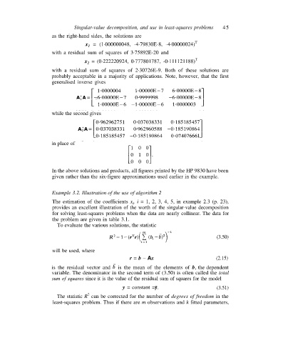
generalised inverse gives

while the second gives

in place of

In the above solutions and products, all figures printed by the HP 9830 have been
given rather than the six-figure approximations used earlier in the example.

Example 3.2. Illustration of the use of algorithm 2
The estimation of the coefficients x , i = 1, 2, 3, 4, 5, in example 2.3 (p. 23),
i
provides an excellent illustration of the worth of the singular-value decomposition
for solving least-squares problems when the data are nearly collinear. The data for
the problem are given in table 3.1.
To evaluate the various solutions, the statistic

(3.50)

will be used, where
r = b – Ax (2.15)

is the residual vector and is the mean of the elements of b, the dependent
variable. The denominator in the second term of (3.50) is often called the total
sum of squares since it is the value of the residual sum of squares for the model
y = constant = (3.51)
2
The statistic R can be corrected for the number of degrees of freedom in the
least-squares problem. Thus if there are m observations and k fitted parameters,