Page 73 - Compact Numerical Methods For Computers

62 Compact numerical methods for computers
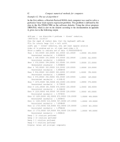
Example 4.2. The use of algorithm 4
In the first edition, a Hewlett-Packard 9830A desk computer was used to solve a
particular linear least-squares regression problem. This problem is defined by the
data in the file EX04.CNM on the software diskette. Using the driver program
DR04.PAS, which is also on the diskette according to the documentation in appendix
4, gives rise to the following output.

dr04.pas -- run Algorithm 4 problems -- Givens’ reduction,
1989/06/03 16:09:47
File for input of control data ([cr] for keyboard) ex04.cnm
File for console image ([cr] = nu1) out04.
alg04. pas -- Givens' reduction, svd, and least squares solution
Order of 1s problem and no. of right hand sides = 51
Enter a number to indicate end of data -9.9900000000E+02
Obsn 1 563.00000 262.00000 461.00000 221.00000 1.00000 305.00000
Uncorrelated residual(s) : 0.0000E+00
Obsn 2 658.00000 291.00000 473.00000 222.00000 1.00000 342.00000
Uncorrelated residual(s) : 0.0000E+00
Obsn 3 676.00000 294.00000 513.00000 221.00000 1.00000 331.00000
Uncorrelated residual(s) : 0.0000E+00
Obsn 4 749.00000 302.00000 516.00000 218.00000 1.00000 339.00000
Uncorrelated residual(s) : 0.0000E+00
Obsn 5 834.00000 320.00000 540.00000 217.00000 1.00000 354.00000
Uncorrelated residual(s) : 0.0000E+00
Obsn 6 973.00000 350.00000 596.00000 218.00000 1.00000 369.00000
Uncorrelated residual(s) : -6.563E-02
Obsn 7 1079.00000 386.00000 650.00000 218.00000 1.00000 378.00000
Uncorrelated residual(s) : -9.733E+00
Obsn 8 1151.00000 401.00000 676.00000 225.00000 1.00000 368.00000
Uncorrelated residual(s) : -6.206E+00
Obsn 9 1324.00000 446.00000 769.00000 228.00000 1.00000 405.00000
Uncorrelated residual(s) : 1.7473E+01
Obsn 10 1499.00000 492.00000 870.00000 230.00000 1.00000 438.00000
Uncorrelated residual(s) : 1.5054E+O1
Obsn 11 1690.00000 510.00000 907.00000 237.00000 1.00000 438.00000
Uncorrelated residual(s) : 7.4959E+00
Obsn 12 1735.00000 534.00000 932.00000 235.00000 1.00000 451.00000
Uncorrelated residual(s) : 1.0754E+00
Obsn 13 1778.00000 559.00000 956.00000 236.00000 1.00000 485.00000
Uncorrelated residual(s) : 1.5580E+O1
Sweep 1 10 rotations performed
Sweep 2 10 rotations performed
Sweep 3 2 rotations performed
Sweep 4 0 rotations performed
Singular values and principal components