Page 74 - Compact Numerical Methods For Computers

Handling larger problems 63

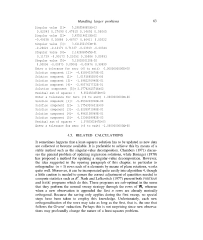
Singular value [1]= 5.2985598853E+03
0.82043 0.27690 0.47815 0.14692 0.00065
Singular value [2]= 3.4551146213Et02
-0.49538 0.30886 0.46707 0.66411 0.00322
Singular value [3]= 3.6112521703E+01
-0.26021 -0.12171 0.71337 -0.63919 -0.00344
Singular value [4]= 2.1420869565E+01
0.11739 -0.90173 0.21052 0.35886 0.00093
Singular value [5]= 5.1382810120E-02
0.00006 -0.00075 0.00045 -0.00476 0.99999
Enter a tolerance for zero (<0 to exit) 0.0000000000E+00
Solution component [1]= -4.6392433678E-02
Solution component [2]= 1.01938655593+00
Solution component [3]= -1.5982291948E-01
Solution component [4]= -2.9037627732E-01
Solution component [5]= 2.0778262574Et02
Residual sum of squares = 9.6524564856E+02
Enter a tolerance for zero (<0 to exit) 1.0000000000E+00
Solution component [1]= -5.8532203918E-02
Solution component [2]= 1.1756920631E+00
Solution component [3]= -2.5228971048E-01
Solution component [4]= 6.9962158969E-01
Solution component [5]= 4.3336659982E-03
Residual sum of squares = 1.0792302647E+03
Enter a tolerance for zero (<0 to exit) -1.0000000000E+00

4.5. RELATED CALCULATIONS

It sometimes happens that a least-squares solution has to be updated as new data
are collected or become available. It is preferable to achieve this by means of a
stable method such as the singular-value decomposition. Chambers (1971) discus-
ses the general problem of updating regression solutions, while Businger (1970)
has proposed a method for updating a singular-value decomposition. However,
the idea suggested in the opening paragraph of this chapter, in particular to
orthogonalise (n + 1) rows each of n elements by means of plane rotations, works
quite well. Moreover, it can be incorporated quite easily into algorithm 4, though
a little caution is needed to ensure the correct adjustment of quantities needed to
2
compute statistics such as R . Nash and Lefkovitch (1977) present both FORTRAN
and BASIC programs which do this. These programs are sub-optimal in the sense
that they perform the normal sweep strategy through the rows of W, whereas
when a new observation is appended the first n rows are already mutually
orthogonal. Because the saving only applies during the first sweep, no special
steps have been taken to employ this knowledge. Unfortunately, each new
orthogonalisation of the rows may take as long as the first, that is, the one that
follows the Givens’ reduction. Perhaps this is not surprising since new observa-
tions may profoundly change the nature of a least-squares problem.