Page 81 - Compact Numerical Methods For Computers

70 Compact numerical methods for computers
When using the singular-value decomposition one could choose to work with
deviations from means or to scale the data in some way, perhaps using columns
which are deviations from means scaled to have unit variance. This will then
prevent ‘large’ data from swamping ‘small’ data. Scaling of equations has proved a
difficult and somewhat subjective issue in the literature (see, for instance, Dahl-
quist and Björck 1974, p 181ff).
Despite these cautions, I have found the solutions to least-squares problems
obtained by the singular-value decomposition approach to be remarkably resilient
to the omission of scaling and the subtraction of means.
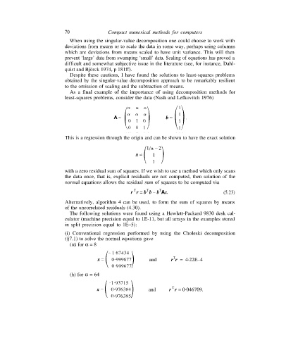
As a final example of the importance of using decomposition methods for
least-squares problems, consider the data (Nash and Lefkovitch 1976)

This is a regression through the origin and can be shown to have the exact solution

with a zero residual sum of squares. If we wish to use a method which only scans
the data once, that is, explicit residuals are not computed, then solution of the
normal equations allows the residual sum of squares to be computed via

T
T
T
r r = b b – b Ax. (5.23)
Alternatively, algorithm 4 can be used, to form the sum of squares by means
of the uncorrelated residuals (4.30).
The following solutions were found using a Hewlett-Packard 9830 desk cal-
culator (machine precision equal to 1E-11, but all arrays in the examples stored
in split precision equal to 1E–5):
(i) Conventional regression performed by using the Choleski decomposition
(§7.1) to solve the normal equations gave
(a) for a = 8

T
and r r = 4·22E–4

(h) for a = 64

T
and r r = 0·046709.