Page 28 - Computational Colour Science Using MATLAB

SOLVING SYSTEMS OF SIMULTANEOUS EQUATIONS 15

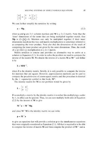
6 1 1 x
.
3 ¼ 1 1 y
We can further simplify the notation by writing

a ¼ Mp, ð2:2Þ

where a and p are 2 1 column matrices and M is a 2 2 matrix. Note that the
‘inner’ dimensions of the terms that are being multiplied together match; thus
Mp is (2 2)(2 1). Matrices can only be multiplied together if their inner
dimensions match in this way and matrix multiplication is sometimes referred to
as computing the inner product. Note also that the dimensions of the result of
computing the inner product are given by the outer dimensions. Thus, the result
of a (2 2)(2 1) multiplication is a 2 1 matrix.
Matrix notation is concise and provides an alternative way to arrive at a
solution to Equation (2.1). In order to solve the problem we need to compute the
inverse of the matrix M. We denote the inverse of a matrix M as M 1 and define
it by

1
I ¼ MM ,

where I is the identity matrix. Strictly, it is only possible to compute the inverse
for matrices that are square. However, approximation methods can be used to
compute the pseudoinverse of a non-square matrix and this procedure is denoted
+
by the + superscript symbol in this book, M .
The identity matrix for M in our problem would be given by

10
.
01
I ¼
If we multiply a matrix by the identity matrix it is rather like multiplying a scalar
by 1; its effect can be ignored. Thus, we can now multiply both sides of Equation
(2.2) by the inverse of M to give

1
1
M a ¼ M Mp,
1
and since M M is the identity matrix we can write
1
p ¼ M a
to give an equation that will provide a solution p to the simultaneous equations
that were originally considered as Equation (2.1). All that is required is to be able
to compute the inverse of matrix M and then compute the product of M 1 and a.