Page 31 - Computational Colour Science Using MATLAB

18 LINEAR ALGEBRA FOR BEGINNERS

x ¼ Ca 1 , ð2:6Þ
where x is the n61 column matrix of X tristimulus values and a is a 3 1 column
1
matrix that will be used to fill the first row of A. Equation (2.6) represents an
over-determined system for n>3 since there are n simultaneous equations and
three variables. Equation (2.6) can be solved by rearranging thus:
1
a 1 ¼ C x, ð2:7Þ
+
where C 1 is replaced by C if n>3. Although it would be possible to solve A for
each row separately, a solution can be found directly from Equation (2.5) to yield
1
A ¼ C T, ð2:8Þ
or, in the more likely case that C is a non-square matrix,
A ¼ C T. ð2:9Þ
þ
Linear algebra can also be used to find non-linear mappings between one set of
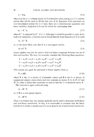
data and another. We may, for example, consider the following three equations:
2
2
2
X ¼ a 11 R þ a 12 G þ a 13 B þ a 14 R þ a 15 G þ a 16 B ,
2
2
2
Y ¼ a 21 R þ a 22 G þ a 23 B þ a 24 R þ a 25 G þ a 26 B ,
2
2
2
Z ¼ a 31 R þ a 32 G þ a 33 B þ a 34 R þ a 35 G þ a 36 B .
This system can again be expressed in linear algebra form as
T ¼ AD, ð2:10Þ
where T is the 36n matrix of tristimulus values and D is the 66n matrix of
2
2
augmented camera values where each row contains six terms: R, G, B, R , G and
2
B . In order to define this transform we need to find the 366 standard matrix A.
The solution is again achieved using
1
A ¼ D T, ð2:11Þ
or, if D is a non-square matrix,
A ¼ D T. ð2:12Þ
þ
Thus, it is evident that very similar methods can be used to determine both linear
and non-linear transforms. In fact, it is reasonable to consider that the linear
transform is simply a special case of a more general set of polynomial transforms.